Machine Learning

18 Apr 2025

Next ↪

---

Table of contents

Intro

Andrew NG has very good courses on machine learning. Many of the below concepts are from those courses, combined with various other sources.

Installing Packages

Installing Anaconda

As first step, download the Anaconda package manager from https://www.anaconda.com. Then follow the installer UI instructions. After a successful installation, open Anaconda-Navigator App.

Installing Jupyter Notebook

From the Anaconda-Navigator, click on Jupyter Notebook Lauch button. Jupyter Notebook will be installed and a webpage will be opend. From now on , you can lauch Jupyter notebook from commandline by typing jypyter-notebook.

Machine Learning

Machine Learning Specialization from Andrew NG is a good reference to understand the basics of Machine learning.

"Machine Learning is the field of study that gives computers the ability to learn withoit being explicitly programmed" - Arutur Samuel 1959

Machine Learning algorithms

• Supervised Machine Learning
  • Regression
  • Classification
• Unupervised Machine Learning
  • Clustering
  • Dimensionality Reduction
• Recommender Systems
  • Netflix recommends movies and shows
• Reinforcement learning
  • Receives rewards or penalties for actions

Supervised Machine Learning- Regression

• The key characteristic of a supervised learning is that you give your learning algorithm examples to learn from.
• These alorithms help to learn input X to output Y mapping
• Examples
  • Smapl filters: X= Email ; Y = Spam (0/1)
  • Speech recognition: X = Audio ; Y = Transcript
  • Machine Translation: X = Englisg; Y = Spanish
  • Online advertising : X = Ad, User-information ; Y = Click (0/1)
  • Self driving car: X = Image, RadarInput; Y = Position of other cars
  • Visual Inspection: X= Image of Phone ; Y = Detect (0/1)
• In all these applications, you will train your model with examples of input X and the expected answers Y (labels)
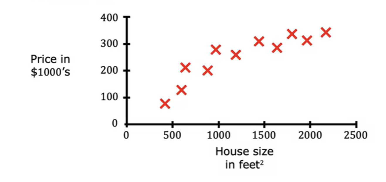
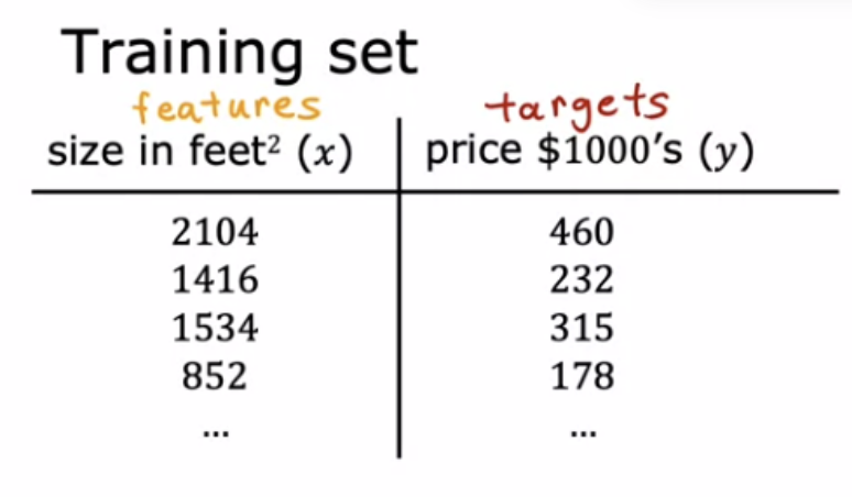
• Example of Housing price based on known data

• Now we have to predict housing price for a new input , say 1200 which is not in the data that we have. You need to find a mathematic function that best fit the data given.
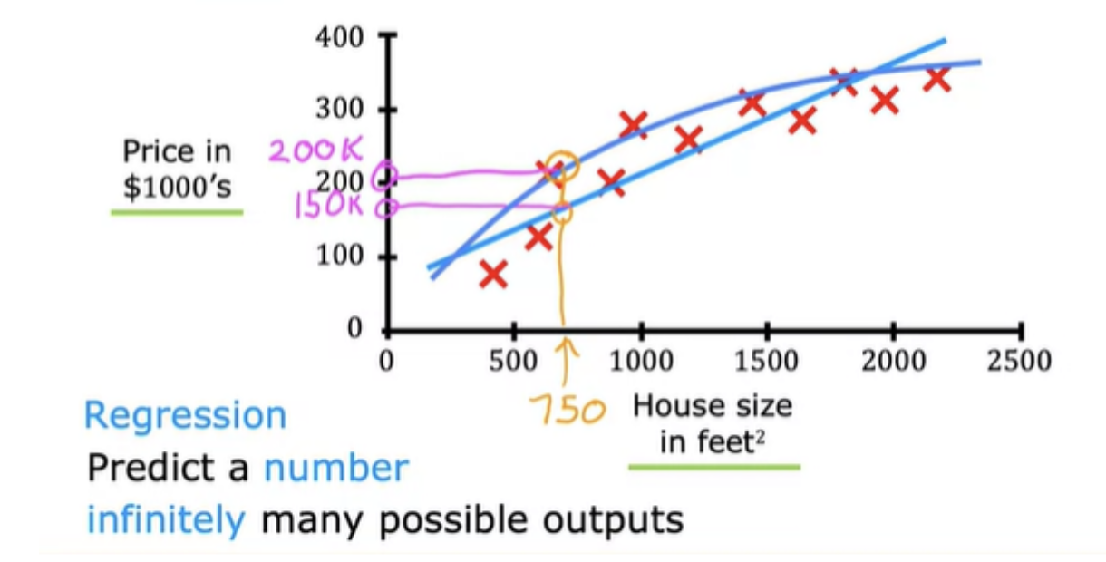
  • For doing this, you need to decide a straight line, a curve or another function that is even more complex for the data.
  • You also need an algorithm to choose the correct function to fit this data.
• This housing price prediction is the particular type of supervised learning called regression. In regression we are trying to predict a number from infinitely many possible numbers, which could be 150,000 or 70,000 or 183,000 or any other number in between.

Supervised Machine Learning- Classification

• Here predict only a small number of output categories (0 or 1 in this case) unlike regression where there are infinitely many.
• Classification predicts categories. It need not to be numbers - it can be non numeric also (predict cat or dog).
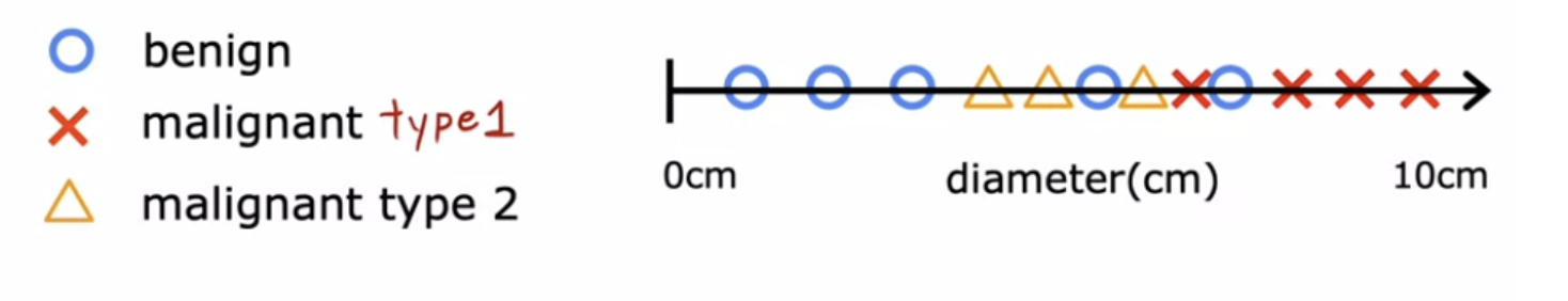
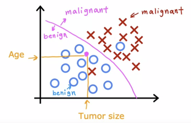
• Example : Identify if given tumor size is benign or not.
• X= input parameters ; Y = Classes or Categories.
• Classification can be more than 2 classes. For example, input parameter is the tumor size, and output classes are benign, malignant type1, and type2.

• You can have also have multiple inputput paramters (X) like age, tumor size.

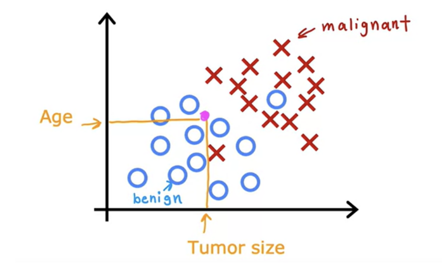
• To do this, algorithm finds some boundary that separates out malignant from benign ones. So the learning algorithm has to decide how to fit a boundary line through this data

Unsupervised learning - Clustering

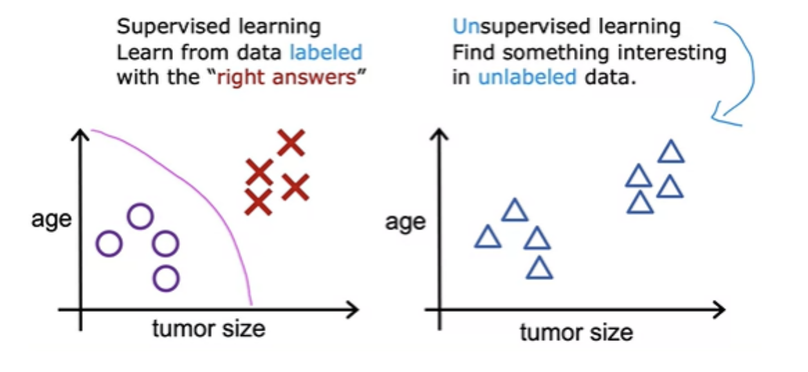
• After supervised learning, the most widely used form of machine learning is unsupervised learning
• In unsupervised learning we are given data that isn't associated with any output labels Y. We dont mark the "right answers" for training the model. We're not asked to diagnose whether the tumor is benign or malignant, because we're not given any labels . Instead, we asked the algorithm to figure out all by yourself what's interesting. The algorithm will output the clusters it sees. This is a particular type of unsupervised learning, called a clustering algorithm that helps to find structure in the data given.

• For example google news groups related news together. This is achived through clustering algorithms. The clustering algorithm figures out what words to use to form a cluster. It can also be used for grouping customers.

Unsupervised learning - Dimensionality Reduction

• Dimensionality reduction lets you take a big data-set and almost magically compress it to a much smaller data-set while losing as little information as possible

More on Linear Regression

• Linear regression is defined as an algorithm that provides a linear relationship between an independent variable (Y) and a dependent variable (X) to predict the outcome of future events. A sloped straight line represents the linear regression model

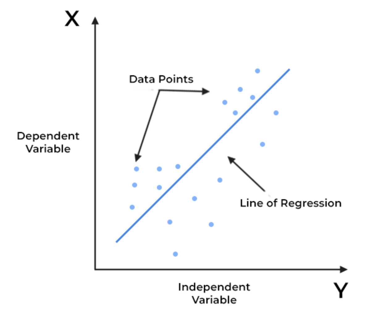
• The linear regression model is computationally simple.

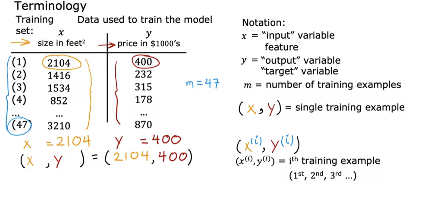
ML Terminology

Linear regression with 1 variable

• To train the model, you feed the training set, both the input features and the output targets to your learning algorithm. Then your supervised learning algorithm will produce some function. Historically, this function used to be called a hypothesis, let us call it a function f . The job with f is to take a new input X and output , and a prediction, which is called Y-hat. In machine learning, the convention is that y-hat is the estimate or the prediction for y.
• The function f is called the model. X is called the input or the input feature and the output of the model is the prediction, Y-hat
• When the symbol is just the letter Y, then that refers to the target, which is the actual true value in the training set. In contrast, Y-hat is an estimate. It may or may not be the actual true value.
• Your model f, given the size, outputs the price which is the estimator, that is the prediction of what the true price will be.

How are we going to represent the function f?

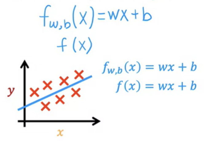
• This function is making predictions for the value of Y using a straight-line function of X. Sometimes you want to fit more complex non-linear functions as well, like a curve. A linear function is relatively simple and easy to work with, and will help you to get to more complex models that are non-linear.
• Above function has a single input variable or feature X, namely the size of the house. This is called a univariate linear regression.

Cost Function

The idea of a cost function is one of the most universal and important ideas in machine learning, and is used in both linear regression and in training many of the most advanced AI models in the world. Take an example of below dataset:

Checking visually with scatterplots or statistically using correlation coefficients we can see that there is a linear relationship between the independent variables (x) and the dependent variable (y). So linear regression could be a choice. In order to implement linear regression the first key step is first to define a cost function. Cost function will tell us how well the model is doing so that we can try to get it to do better

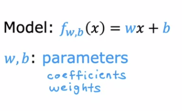
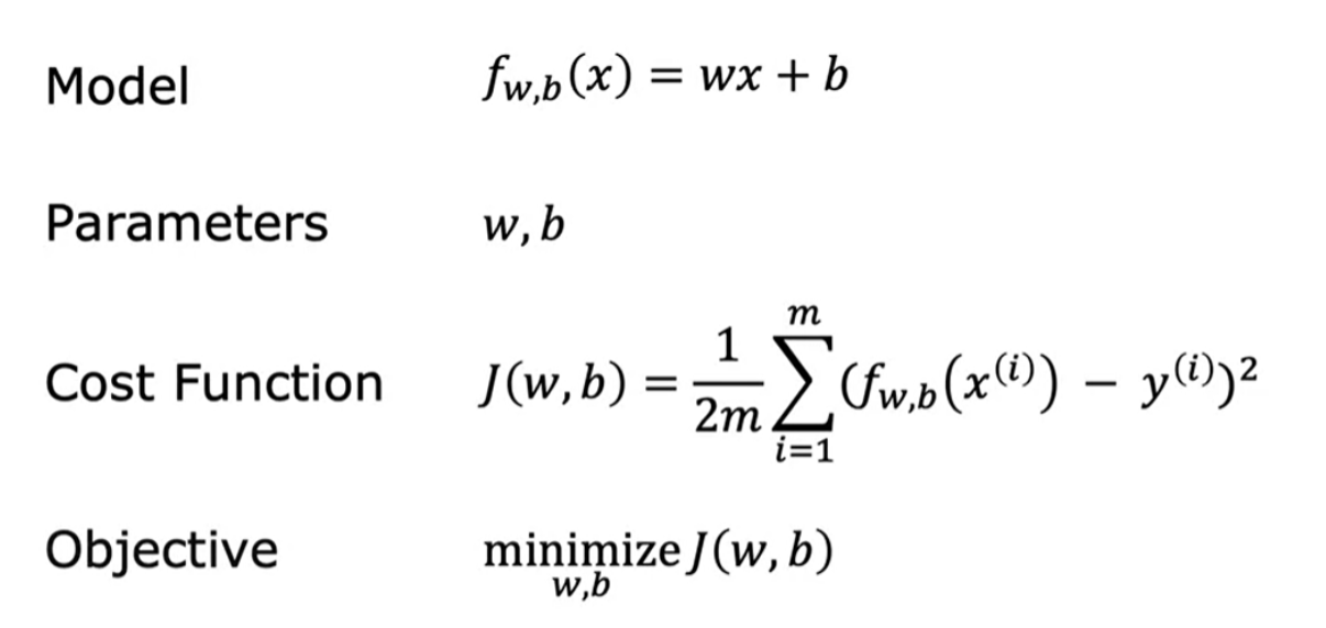
The model we are going to choose is a function above, where w and b are parameters (coefficients / weights). Depending on the values you've chosen for w and b you get a different function f of x, which generates a different line on the graph

• f(x) = 0x + 1.5
• f(x) = 0.5x + 0
• f(x) = 0.5x + 1

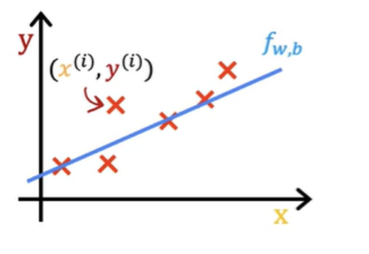
With linear regression, you want choose values for the parameters w and b so that the straight line you get from the function f somehow fits the data well

Finding values for w and b

How to automatically find the value of w and b? From the training data you have:

• y⁽¹⁾ , x⁽¹⁾
• y⁽²⁾ , x⁽²⁾
• y⁽³⁾ , x⁽³⁾

Predicting the the values (ŷ) using the model formula y= w*x + b :

• ŷ⁽¹⁾ = x⁽¹⁾ + b
• ŷ⁽²⁾ = x⁽²⁾ + b
• ŷ⁽³⁾ = x⁽³⁾ + b

In above formula you used one of the w and b values. There are other w and b values you have to try. You have to find best value for w and b so that the the prediction ŷ is close to the training y value, for all training samples. To do that, you need to construct a cost function.

Cost function defintion

The cost function takes the prediction ŷ and compares it to the target y by taking (ŷ - y). This difference is called the error. Here we are measuring how far off to prediction is from the target. We use squared eror to avoid negative and positves mixup.

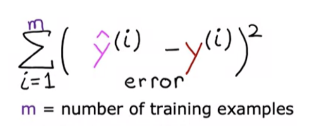
Notice that if we have more training examples (m) is larger, and your cost function will calculate a bigger number since it is summing over more example. To build a cost function that doesn't automatically get bigger as the training set size gets larger we do below:

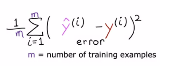
By convention, the cost function that machine learning people use actually divides by 2 times m. The extra division by 2 is just meant to make some of our later calculations look neater, but the cost function still works whether you include this division by 2 or not

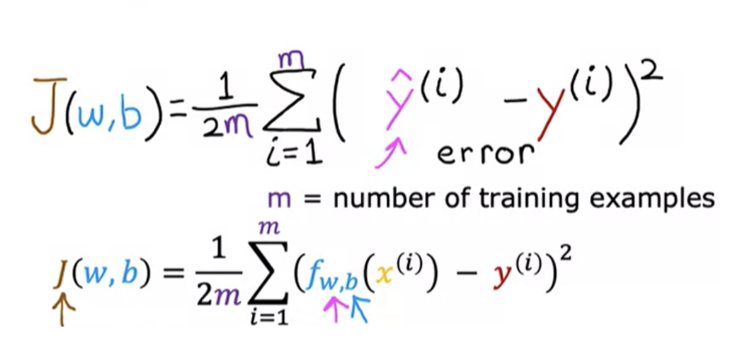
In machine learning different people will use different cost functions for different applications, but the squared error cost function is by far the most commonly used one for linear regression

We have to find values of w and b that make the cost function small (ie, find best parameters for your model). Linear regression would try to find values for w, and b, that make a J(w,b) be as small as possible. For example: J (0.5,0) = 0.58

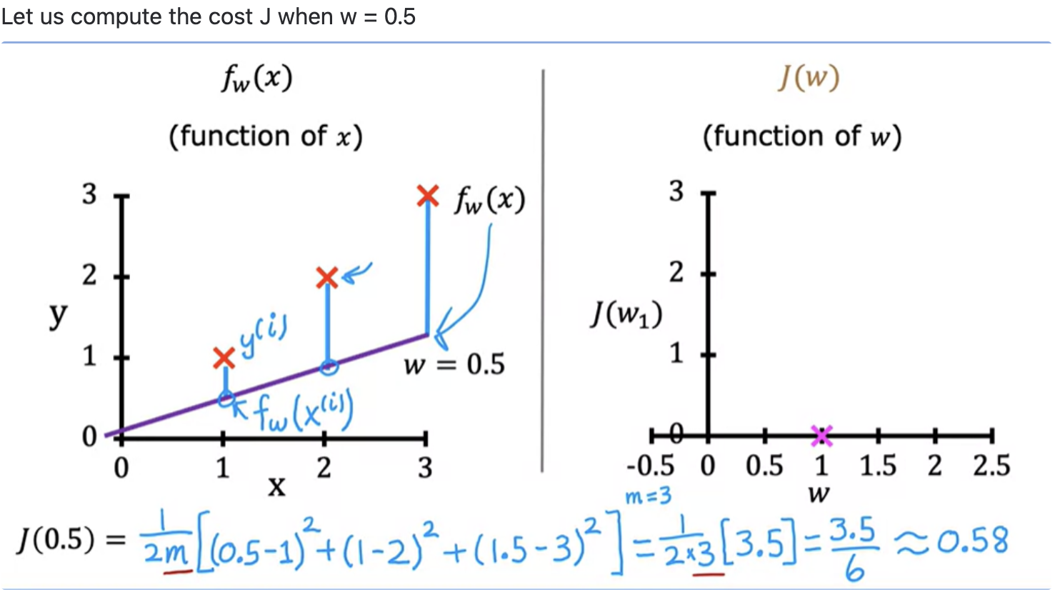
Minimising cost function - Example using single parameter

Let us consider a cost function J with single parameter w. It is unlikely that the initial J(w) yoou tried gives the minimu possible value of J. Increment the values of (w and b) in a sequence, and plot corresponding J values. By computing a range of values, you can slowly trace out the cost function J :

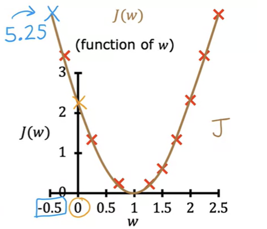
Choosing a value of w and b that causes J (w) to be as small as possible is a good model. In other words, find the values of w and b that minimize J.

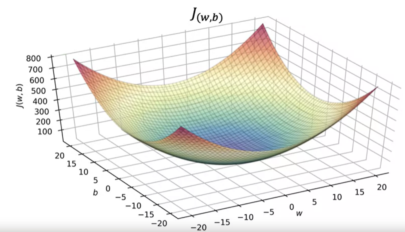
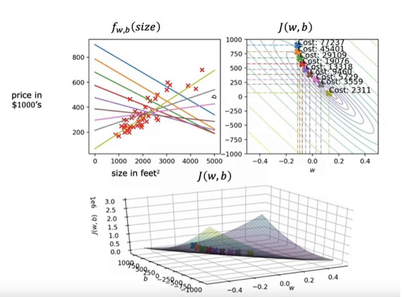
Cost function with more parameters

It is easy to plot when there is 1 parameter (w) . It is complex to plot J since there are 2 parameters (w and b). It turns out that the cost function shape like a soup bowl, except in three dimensions instead of two.

The plot of cost fuinction (for a range of J values) is below:

Alternate way of plotting cost function

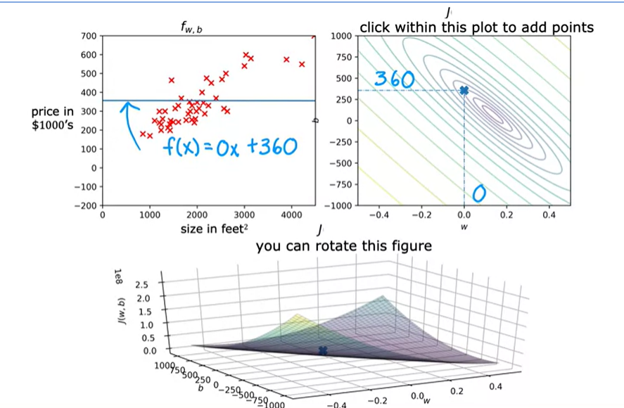
There's another way of plotting the cost function J which is, rather than using these 3D-surface plots. We can plot it using something called a contour plot

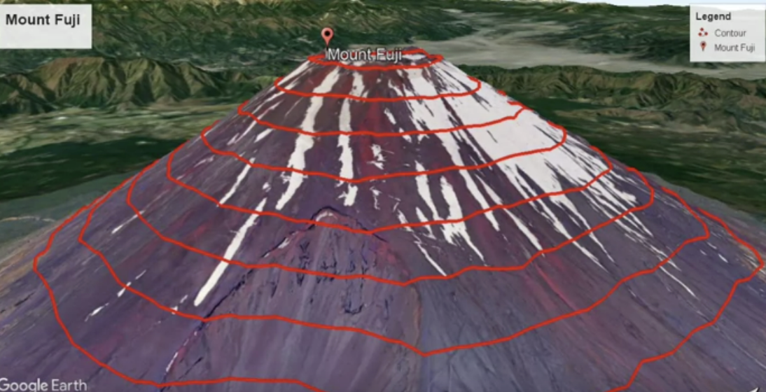
All of the points in a ring will have the same value for the cost function J, even though they have different values for w and b. b=0, w = 360 example

What you really want is an efficient algorithm that automatically finds the values of parameters w and b that give you the best fit line that minimizes the cost function J. There is an algorithm for doing this (training model) called gradient descent. This is one of the most important algorithms in machine learning. It is not just linear regression, but also used in some of the biggest and most complex models in all of AI.

x_train = np.array([1.0, 2.0])        #(size in 1000 square feet)
y_train = np.array([300.0, 500.0])    #(price in 1000s of dollars)


def compute_cost(x, y, w, b): 
    """
        Computes the cost function for linear regression.

        Args:
          x (ndarray (m,)): Data, m examples 
          y (ndarray (m,)): target values
          w,b (scalar)    : model parameters  

        Returns
            total_cost (float): The cost of using w,b 
            as the parameters for linear regression
            to fit the data points in x and y
    """
    
    # number of training examples
    m = x.shape[0] 
    
    cost_sum = 0 
    for i in range(m): 
        f_wb = w * x[i] + b   
        cost = (f_wb - y[i]) ** 2  
        cost_sum = cost_sum + cost  
    total_cost = (1 / (2 * m)) * cost_sum  

    return total_cost

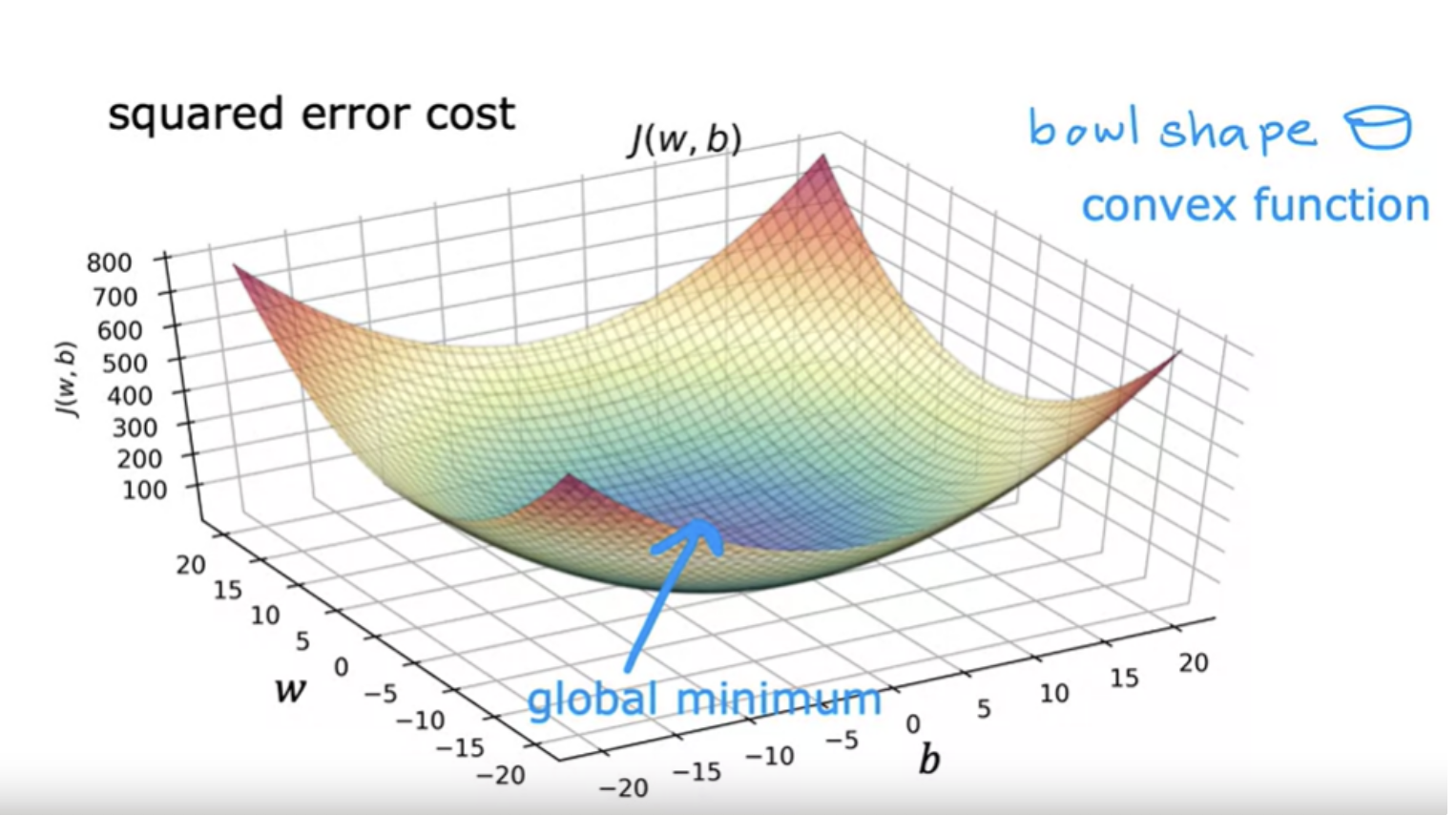
The fact that the cost function squares the loss ensures that the 'error surface' is convex like a soup bowl. It will always have a minimum that can be reached by following the gradient in all dimensions.

Gradient descent

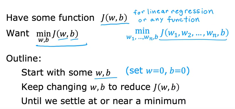
Gradient descent is a systematic way to find the values of w and b, that results in the smallest possible cost. Gradient descent is used all over the place in machine learning, not just for linear regression, but for training of the most advanced neural network models, also called deep learning models. Gradient descent is an algorithm that you can use to try to minimize any function, not just a cost function for linear regression - gradient descent more general.

Start off with some initial guesses of w and b. In linear regression, it won't matter too much what the initial value are, so a common choice is to set them both to 0. For example, you can set w to 0 and b to 0 as the initial guess.

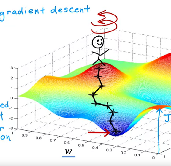
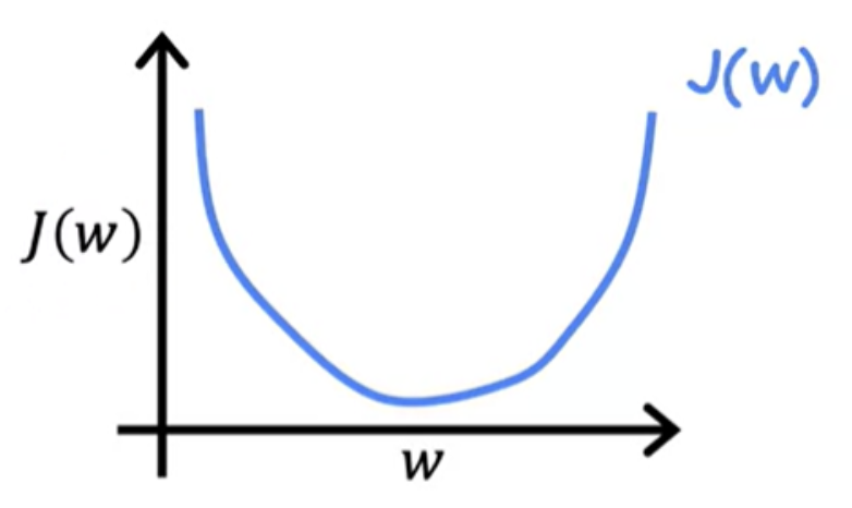
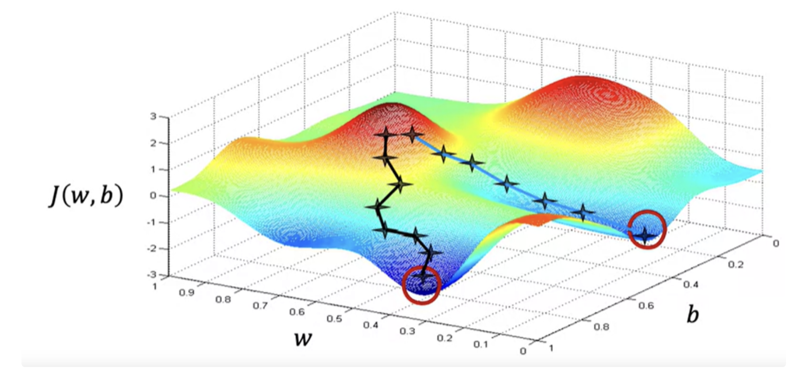
For linear regression with the squared error cost function, you always end up with a bow shape or a hammock shape. Some J functions may not be a bow shape or a hammock shape, it is possible for there to be more than one possible minimum (not a squared error cost function). This is a type of cost function you might get if you're training a neural network model. Your goal is to start up here and get to the bottom of one of these valleys as efficiently as possible by taking small steps.

gradient descent has an interesting property- If you were to run gradient descent this second time, starting just a couple steps in the right of where we did it the first time, then you end up in a totally different valley

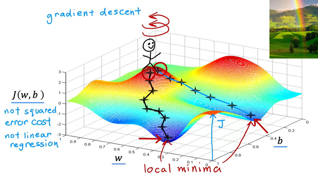
Because if you start going down the first valley, gradient descent won't lead you to the second valley, and the same is true if you started going down the second valley- you stay in that second minimum and not find your way into the first local minimum

Implementing gradient descent

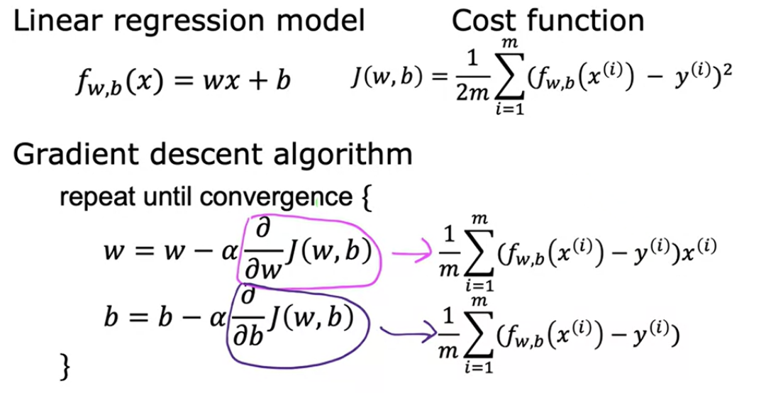
On each step, w, the parameter, is updated as below. You're trying to minimize the cost by adjusting the parameter w.

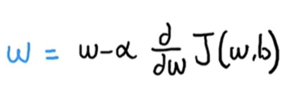
Alpha (learning rate) basically controls how big of a step you take downhill.

You need to do the same for second parameter b as well

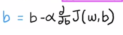
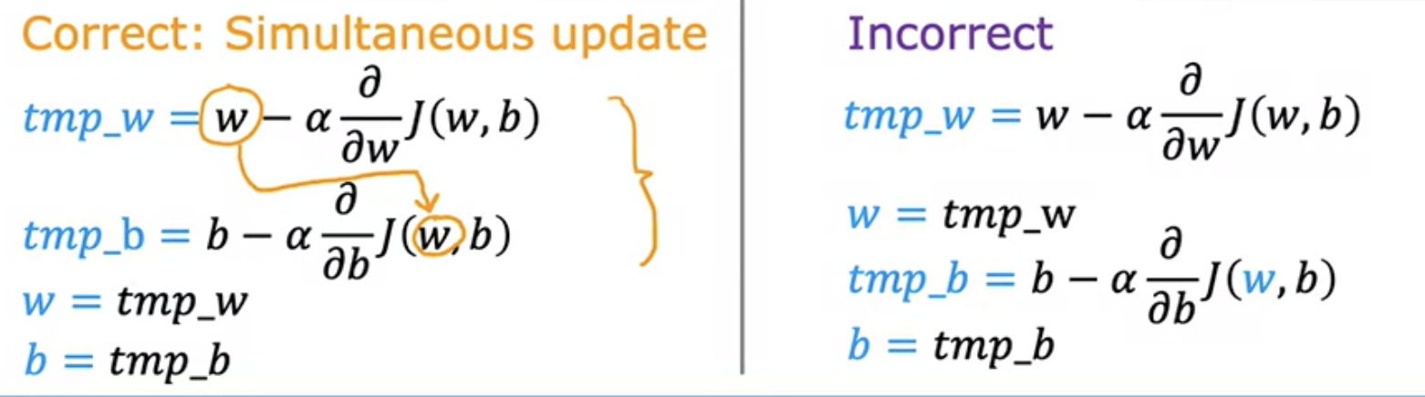
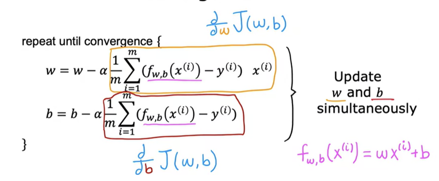
You have to repeat this until convergence. It means that you reach the point at a local minimum where the parameters w and b no longer change much with each additional step that you take. This update takes place for both parameters, w and b. you want to simultaneously update w and b.

Derivative vs partial derivative

Above formula used partial derivative. But for the purposes of implementing a machine learning algorithm we may callit just derivative.

In mathematics, sometimes the function depends on two or more variables. partial derivative is the derivative of a function of several variables with respect to change in just one of its variables. Partial derivatives are useful when dealing with functions of multiple variables like in economics where systems depend on several factors. For example, in a function representing the temperature of a room as a function of both time and position, we might want to know how temperature changes at a specific point with respect to time, holding the spatial coordinates constant. Suppose, we have a function f(x, y), which depends on two variables x and y, where x and y are independent of each other. Then we say that the function f partially depends on x and y

A total derivative, also known as a full derivative, accounts for the changes in all variables of a function simultaneously. It describes how the function changes as all its variables change. Example, in a function representing the position of an object as a function of time, the total derivative would describe how position changes with respect to time, taking into account all factors affecting position. For one variable functions, partial derivative is the same as total derivative

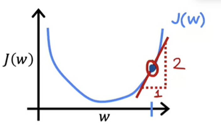
Derivative using cost function graph

A way to think about the derivative at this point on the line is to draw a tangent line, which is a straight line that touches this curve at that point. The slope of this line is the derivative of the function J at this point. To get the slope, you can draw a little triangle. If you compute the height divided by the width of this triangle, that is the slope. For example, this slope might be 2/1. For instance and when the tangent line is pointing up and to the right, the slope is positive, which means that this derivative is a positive number, so is greater than 0.

The learning rate is always a positive number. If you take w minus a positive number, you end up with a new value for w, that's smaller

Choice of learning rate

The choice of the learning rate, alpha will have a huge impact on the efficiency of your implementation of gradient descent. And if the learning rate is chosen poorly rate of descent may not even work at all.

If Alpha is very small, then you'd be taking small baby steps downhill.When too small, then gradient descents will work, but it will be slow.

If Alpha is very large, then that corresponds to a very aggressive gradient descent procedure where you're trying to take huge steps downhill. The gradient descent may overshoot and may never reach the minimum.

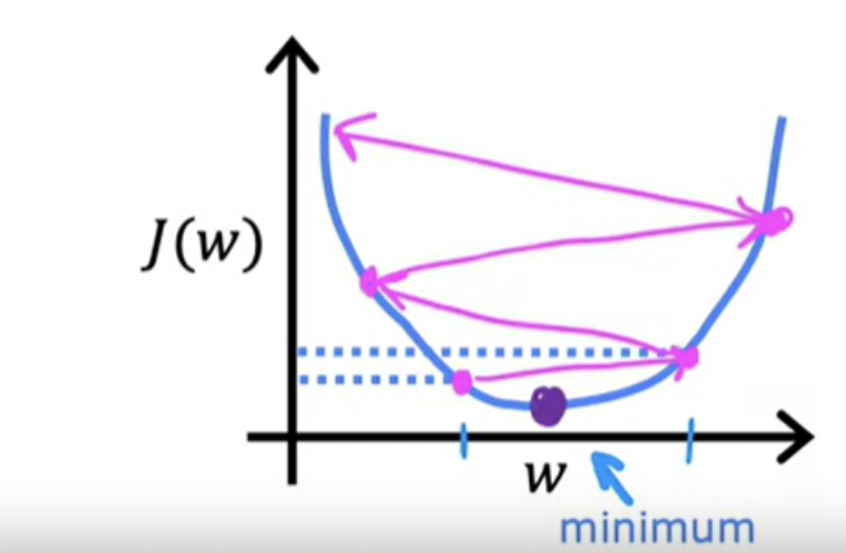
As shown in figure, you are actually already pretty close to the minimum. But if the learning rate is too large then you update W very giant step to be all the way over here. you take another huge step with an acceleration and way overshoot the minimum again. So if the learning rate is too large, then gradient descent may overshoot and may never reach the minimum. And another way to say that is that gradient descent may fail to converge, and may even diverge.

Starting point at a local minimum

What One step of gradient descent will do if one of your parameter w is already at a point so that your cost J is already at a local minimum ?

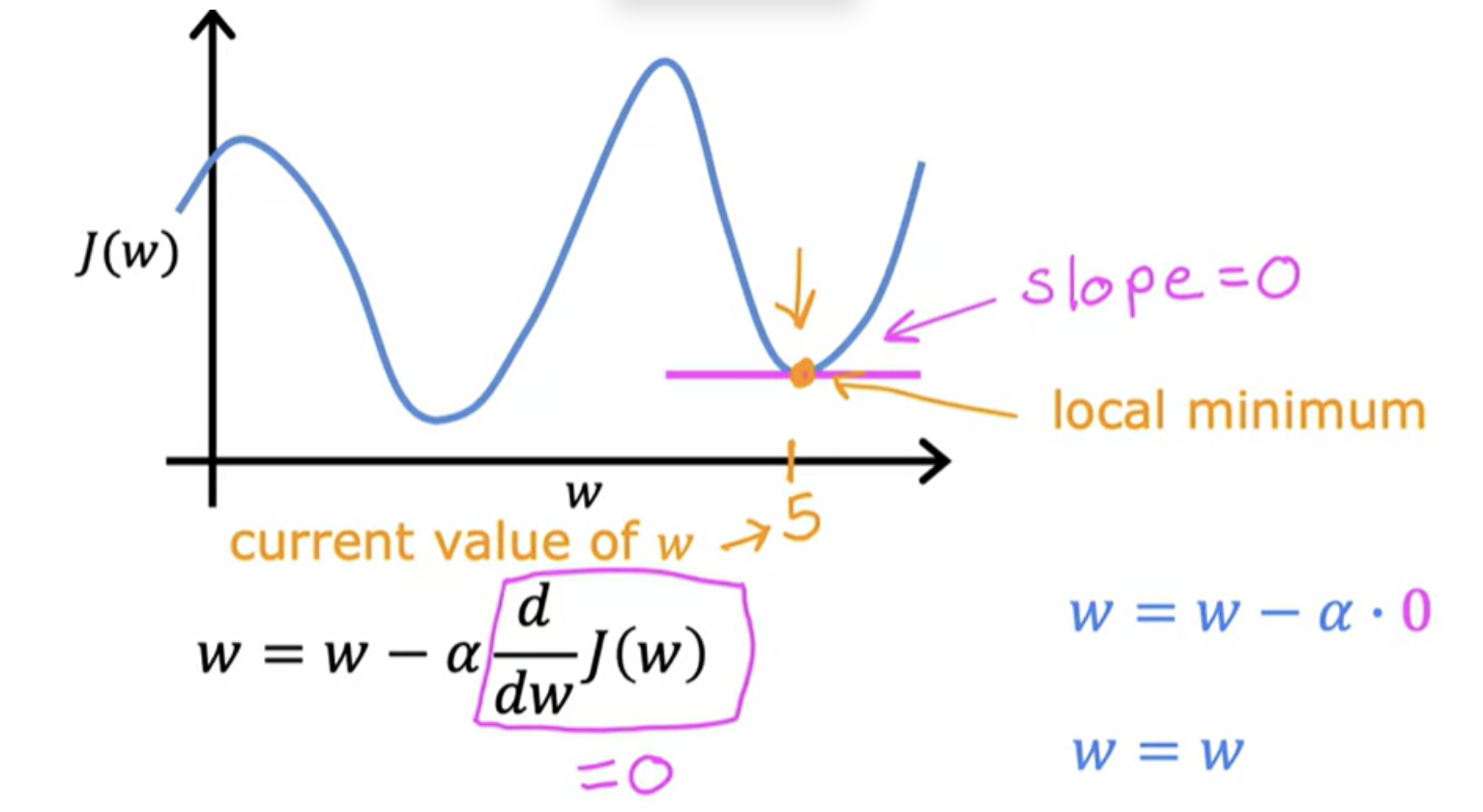
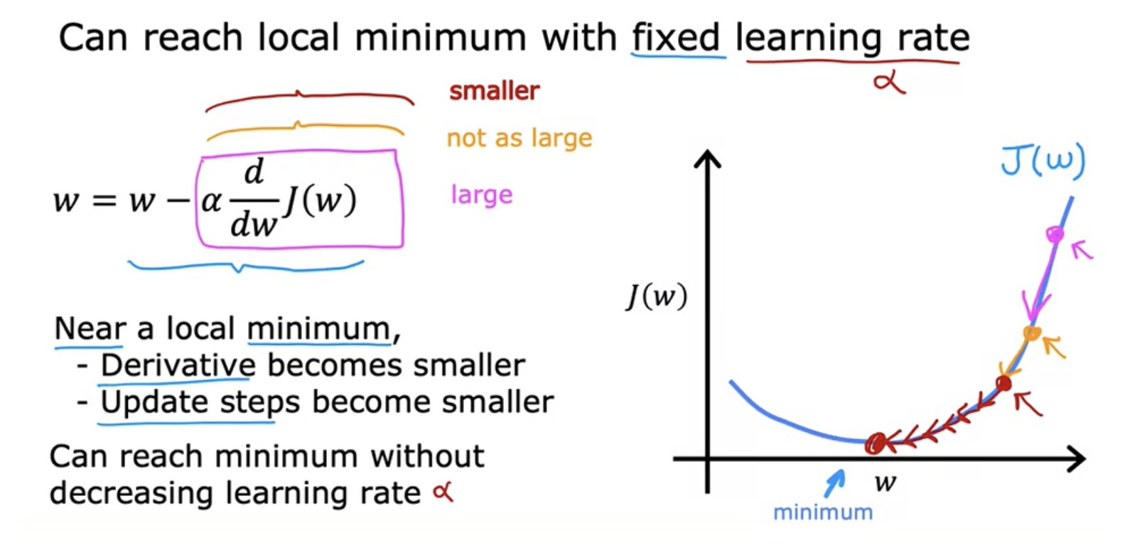
At local minimum, derivative of J be equal to zero for the current value of w. So this means that if you're already at a local minimum, gradient descent leaves w unchanged. So it just updates the new value of W to be the exact same old value of w. So if your parameters have already brought you to a local minimum, then further gradient descent steps to absolutely nothing. This also explains why gradient descent can reach a local minimum, even with a fixed learning rate alpha.

Near local minimum, the derivative of J becomes smaller, update steps become smaller. As we get nearer a local minimum gradient descent will automatically take smaller steps. Update steps also automatically gets smaller even if the learning rate alpha is kept at some fixed value. So it can reach local minium without decreasing the learning rate alpha.

Gradient descent for linear regression

More than one local minimum

One issue we saw with gradient descent is that it can lead to a local minimum instead of a global minimum. Global minimum is the point that has the lowest possible value for the cost function J of all possible points. Depending on where you initialize the parameters w and b, you can end up at different local minima. For example, neural networks.

But when you're using a squared error cost function with linear regression, the cost function does not and will never have multiple local minima. It has a single global minimum because of this bowl-shape. The technical term for this is that this cost function is a convex function. When you implement gradient descent on a convex function, one nice property is that so long as you're learning rate is chosen appropriately, it will always converge to the global minimum.

Running gradient descent for linear regression

Batch gradient descent

The term batch gradient descent refers to the fact that on every step of gradient descent, we're looking at all of the training examples, instead of just a subset of the training data. ie, batch gradient descent is looking at the entire batch of training examples at each update. It is an optimization algorithm

The term “batch gradient descent” is actually what many people casually refer to as just “gradient descent”. In practice, the term "gradient descent" is a general umbrella that includes several variants based on how much data is used for each update.

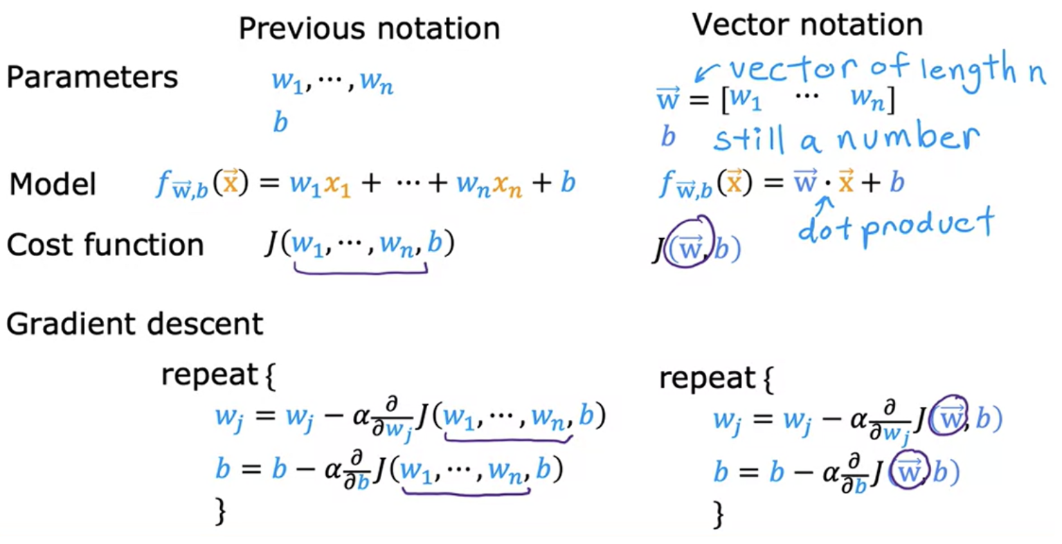
Regression with multiple input variables

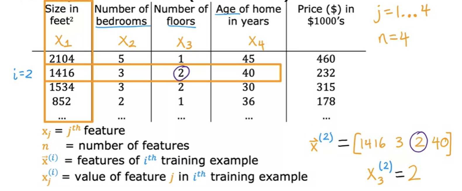
In linear regression example, you had a single feature x (size of the house) and you're able to predict y (the price of the house). But there can be other parameters also like number of bedrooms, number of floors, age of the house etc. This will give you a lot more information with which to predict the price.

This is sometimes this is called a row vector. We will draw an arrow on top of that to indicate that it is a vector. The corresponding model for this will be:

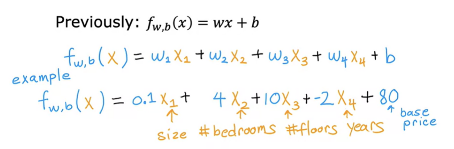
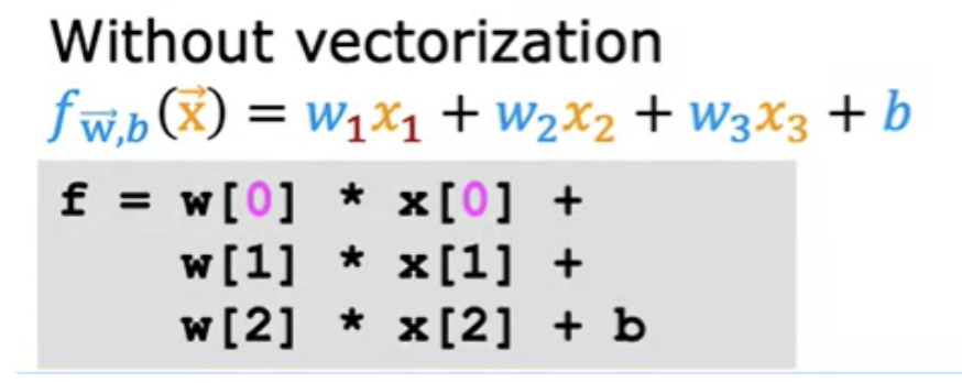
In general, if you have n features, then the model will look like:

• f _w,b = w₁x₁ + w₁x₁ + w₂x₂ + w₃x₃ + ... + w_nx_n + b

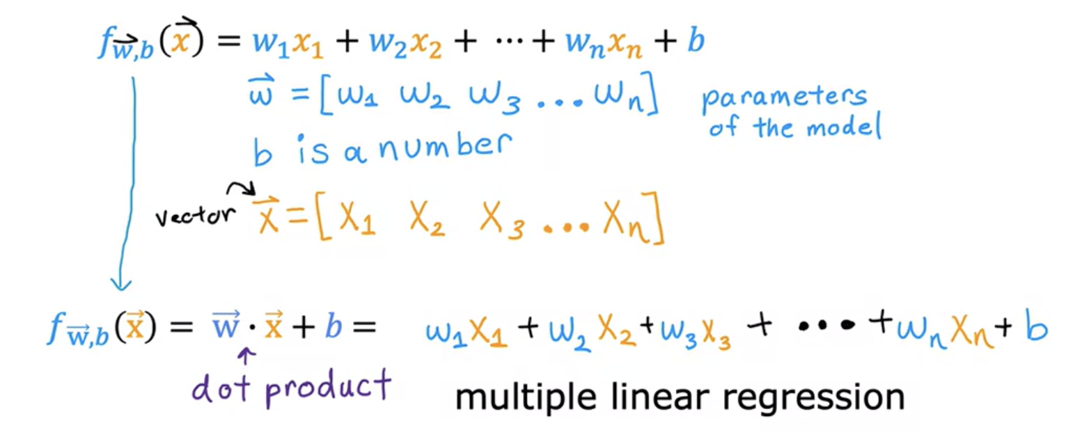
The name for this type of linear regression model with multiple input features is multiple linear regression. This is in contrast to univariate regression, which has just one feature. Multiple linear regression is probably the single most widely used learning algorithm in the world today.

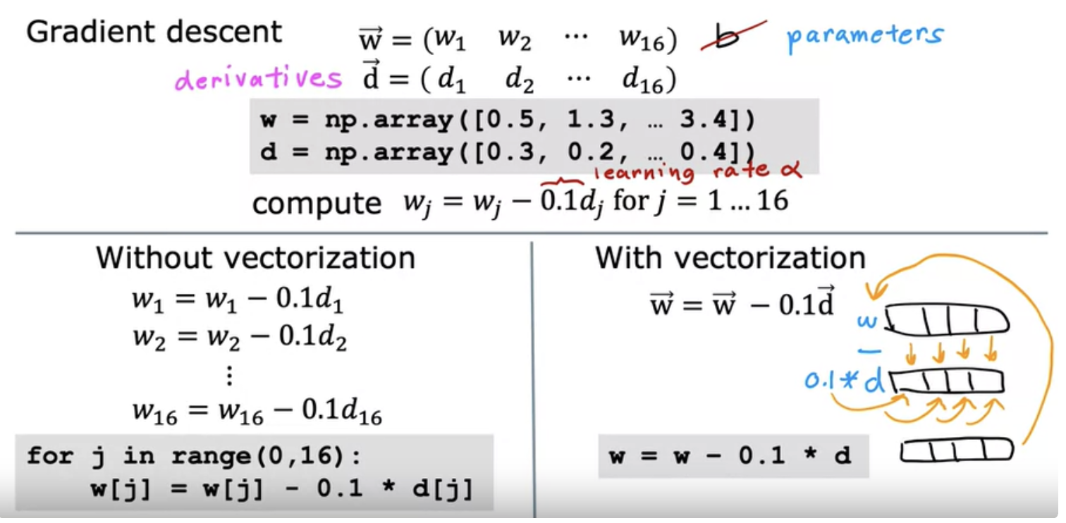
Vectorization

When you're implementing a learning algorithm, using vectorization will both make your code shorter and also make it run much more efficiently. Learning how to write vectorized code will allow you to also take advantage of modern numerical linear algebra libraries, as well as GPU hardware.

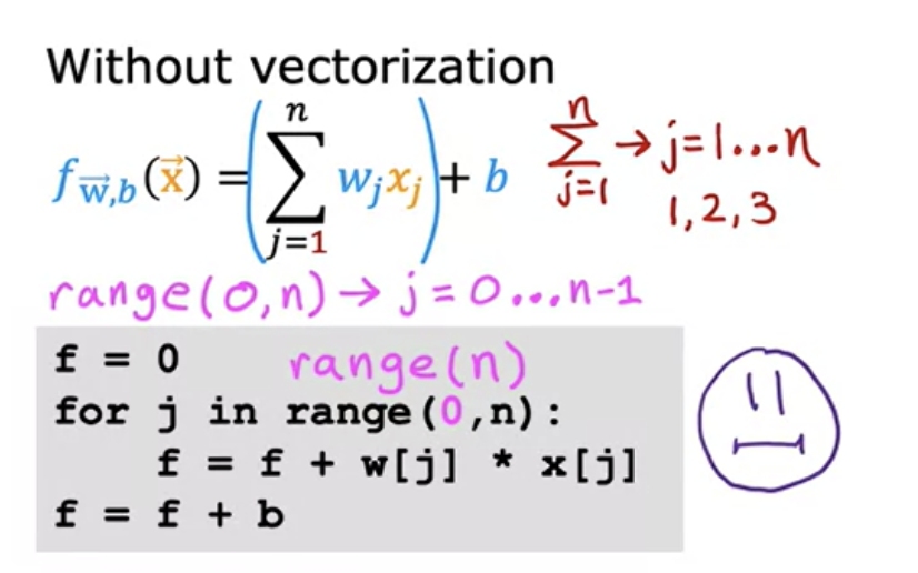
When n become large like 1000, the computation will become inefficient. May be we can use a efficient python syntax like like below one to improve it a but further:

But if we vectorize, it will look like below:

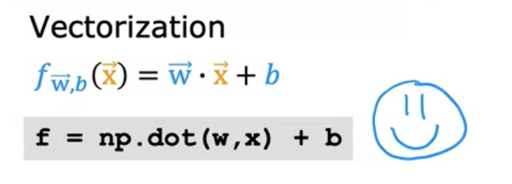
This NumPy dot function is a vectorized implementation of the dot product operation between two vectors and especially when n is large, this will run much faster than the two previous code examples. Vectorisation makes code shorter and efficient. The NumPy dot function is able to use parallel hardware in your computer. This is true whether you're running this on a normal computer CPU or a GPU

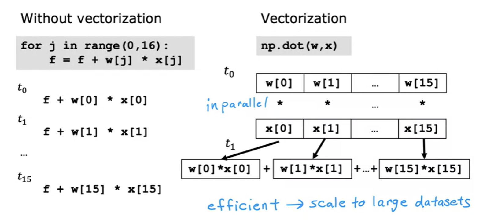
The computer can get all values of the vectors w and x, and in a single-step, it multiplies each pair of w and x with each other all at the same time in parallel. After that, the computer takes these 16 numbers and uses specialized hardware to add them altogether very efficiently, rather than needing to carry out distinct additions one after another. This helps in efficient implementation of multiple linear regression gradient discent, for example.

Vector representation

Vectors are denoted with lower case bold letters such as x_x. The elements of a vector are all the same type. A vector does not, for example, contain both characters and numbers. The number of elements in the array is often referred to as the dimension.

NumPy and python work together fairly seamlessly. Python arithmetic operators work on NumPy data types and many NumPy functions will accept python data types.

Vectorised Gradient descent for multiple linear regression

Normal equation

Normal equation is an alternative way for finding w and b for linear regression. Almost no machine learning practitioners should implement the normal equation method. But if you're using a mature machine learning library and call linear regression, there is a chance that on the backend, it'll be using Normal equation to solve for w and b. Normal equation works only in linear regression case. It also slow when. number of features are large like more than 10,000.

---

Next ↪