Consider below model for housing price
Applying the largest feature range (2000 and 5) into the model, with model parameters w(1) = 50 , w(2)= 0.1 , b = 50 :
Another example with w(1) = 0.1 , w(2)= 50 , b = 50 :
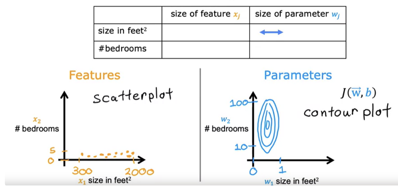
When the possible range of values of a feature is large a good model will learn to choose a relatively small parameter value, like 0.1. Likewise, when the possible values of the feature are small then a reasonable parameter value will be relatively large like 50.
The contour plot has the horizontal axis has a much narrower range, say between zero and one, whereas the vertical axis takes on much larger values, say between 10 and 100. So the contours form ovals or ellipses. This is because a very small change to w1 can have a very large impact on the estimated price and that's a very large impact on the cost J.
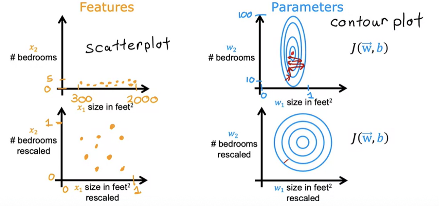
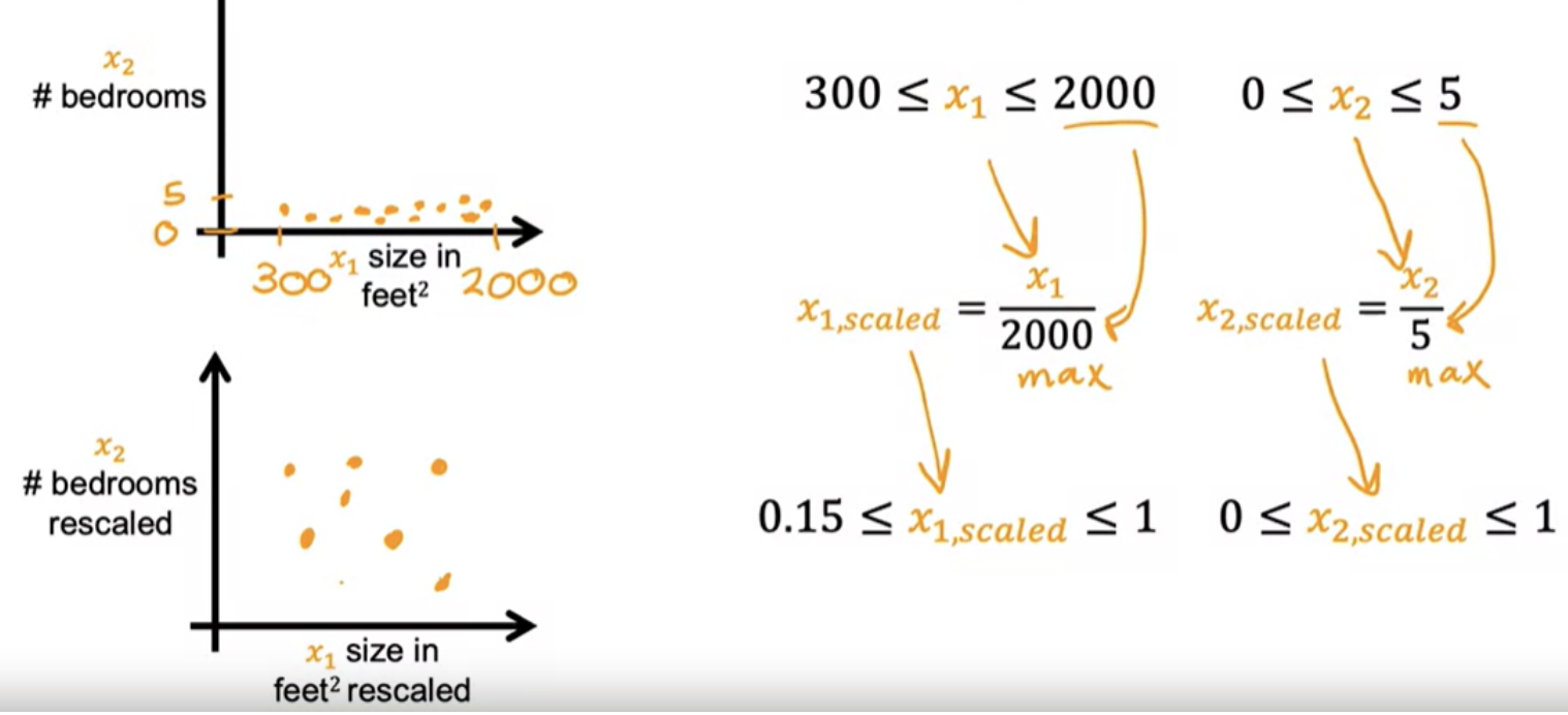
Because the contours are so tall and skinny, gradient descent may end up bouncing back and forth for a long time before it can finally find its way to the global minimum. In situations like this, a useful thing to do is to scale the features.This means performing some transformation of your training data so that x 1 say might now range from 0 to 1 and x2 might also range from 0 to 1.
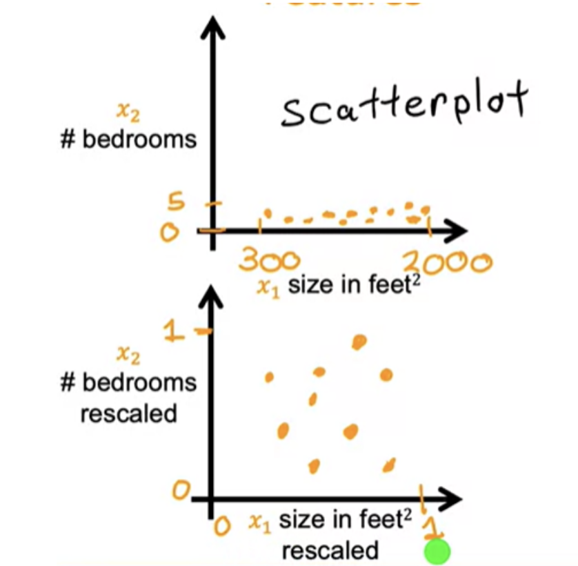
When you have different features that take on very different ranges of values, it can cause gradient descent to run slowly but re scaling the different features so they all take on comparable range of values. After rescaling, gradient descent can find a much more direct path to the global minimum.
The key point is that the re-scaled x 1 and x 2 are both now taking comparable ranges of values to each other. If you run gradient descent on a cost function, contours will look more like this more like circles and less tall and skinny.
One of the option to scale is dividing by the maximum
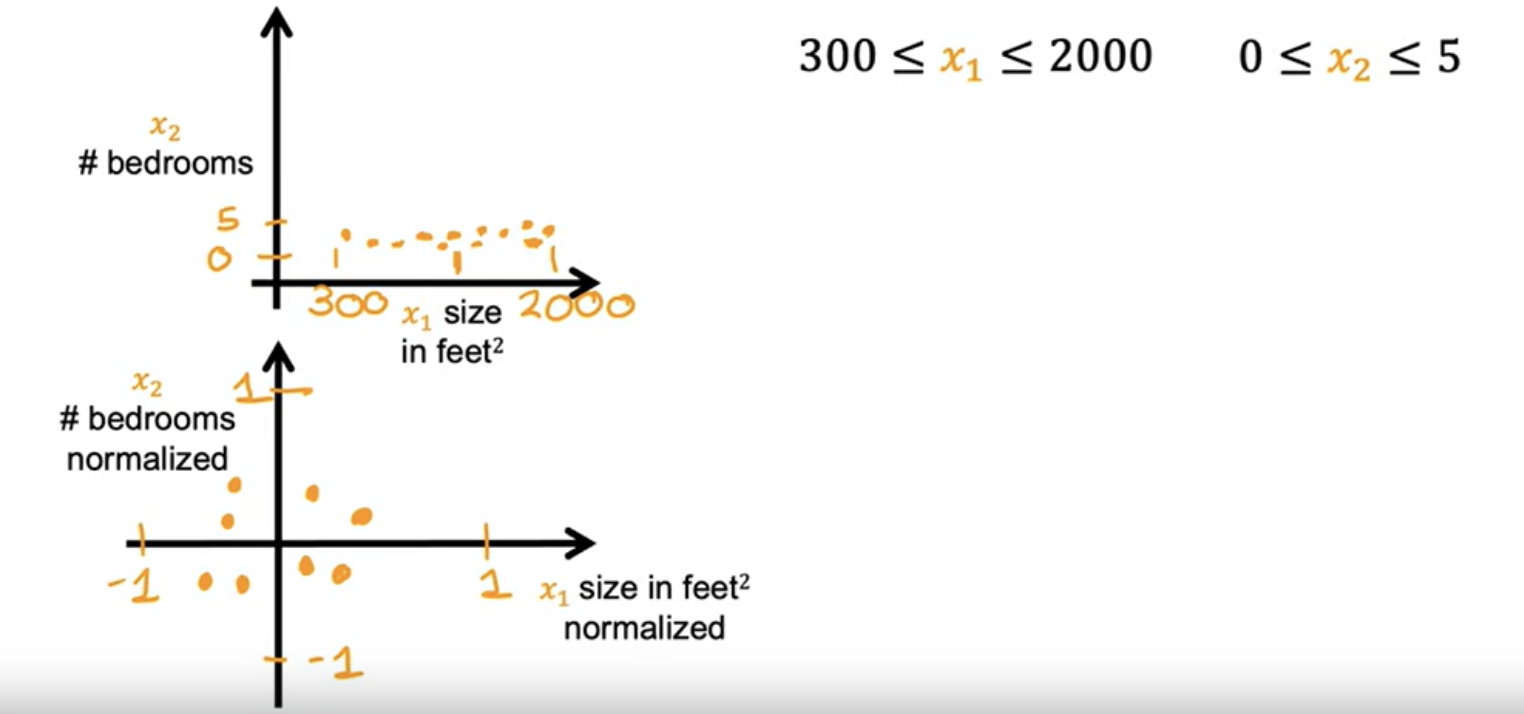
The other option to scale is mean normalization
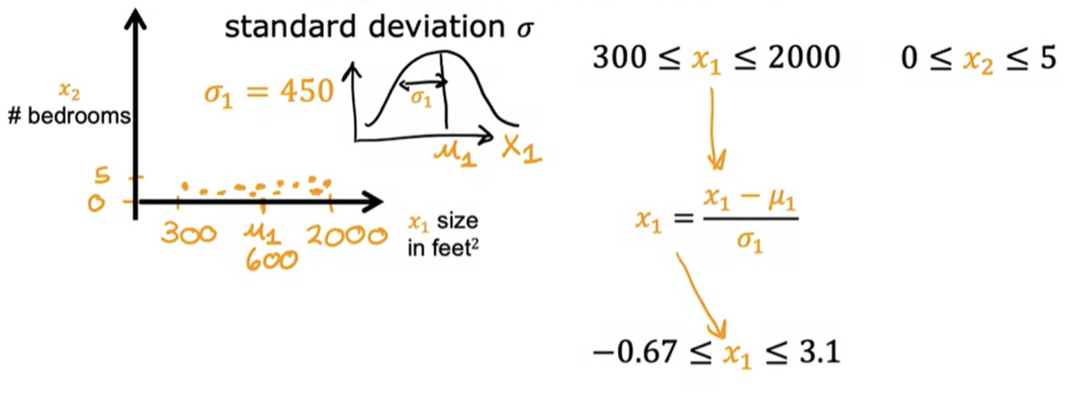
Yet other option to scale is z-score normalization
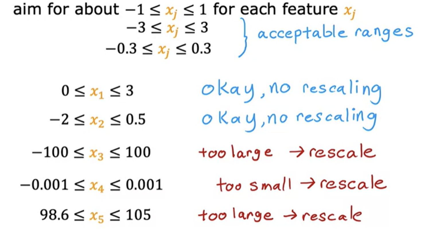
There's almost never any harm to carrying out feature re-scaling. When in doubt, you to just carry it out
Following is an example of cases where feature scaling can be applied.In this example, x5 representing temperature values are around 100, which is actually pretty large compared to other scale features, and this will actually cause gradient descent to run more slowly. In this case, feature re-scaling will help.
The job of gradient descent is to find parameters w and b that hopefully minimize the cost function J. But when running gradient descent, how can you tell if it is converging?
Plotting the value of J at each iteration of gradient descent (Learning curve):
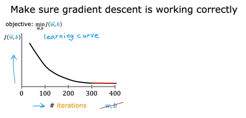
After you've run gradient descent for 100 iterations, (100 simultaneous updates of the parameters), look into the curve to see how your cost J changes after each iteration. If gradient descent is working properly, then the cost J should decrease after every single iteration. If J ever increases after one iteration, that means either Alpha is chosen poorly, and it usually means Alpha is too large, or there could be a bug in the code.
Another obersation is that by the time you reach 300 iterations, the cost J is leveling off and is no longer decreasing much. By 400 iterations, it looks like the curve has flattened out. Looking at this learning curve, you can try to spot whether or not gradient descent is converging.
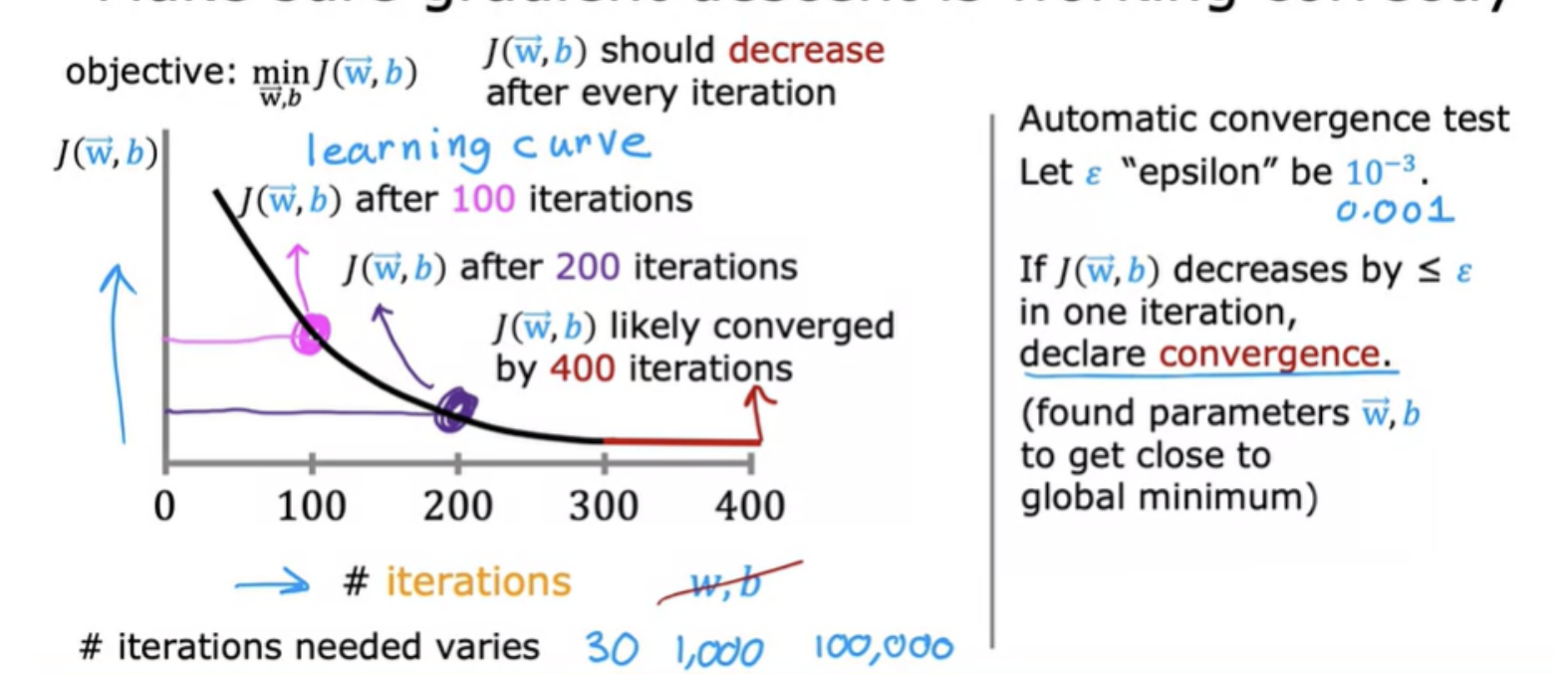
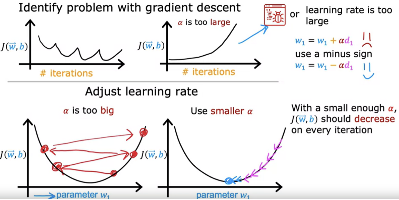
We can actually look at graphs like this rather than rely on automatic convergence tests. If learning rate is too small, it will run very slowly and if it is too large, it may not even converge.
If you plot the cost for a number of iterations and notice that the costs sometimes goes up and sometimes goes down, you should take that as a clear sign that gradient descent is not working properly.
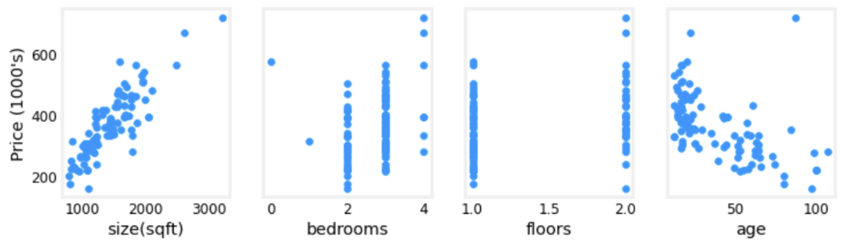
The choice of features can have a huge impact on your learning algorithm's performance. Choosing or entering the right features is a critical step to making the algorithm work well
For example plotting each feature vs. the target, price, provides some indication of which features have the strongest influence on price. Bedrooms and floors don't seem to have a strong impact on price. Newer houses have higher prices than older houses:
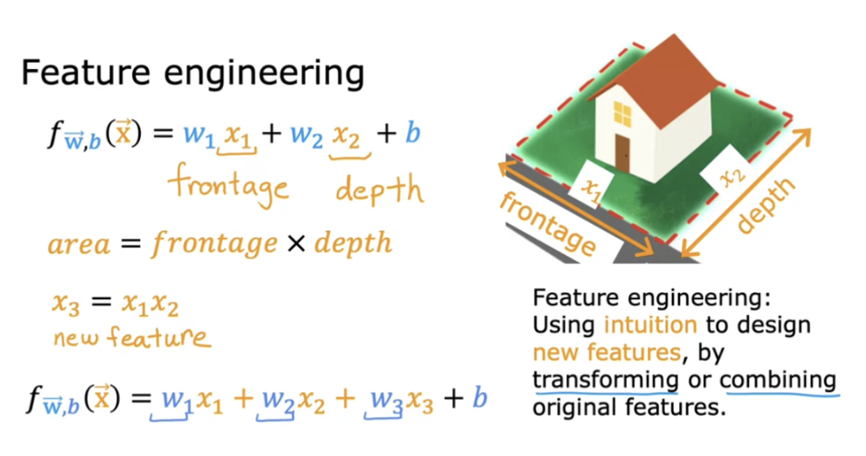
Feature engineering - using intuition to design new features by transforming or combining original features. Depending on what insights you may have into the application, you may define new features, and get a much better model
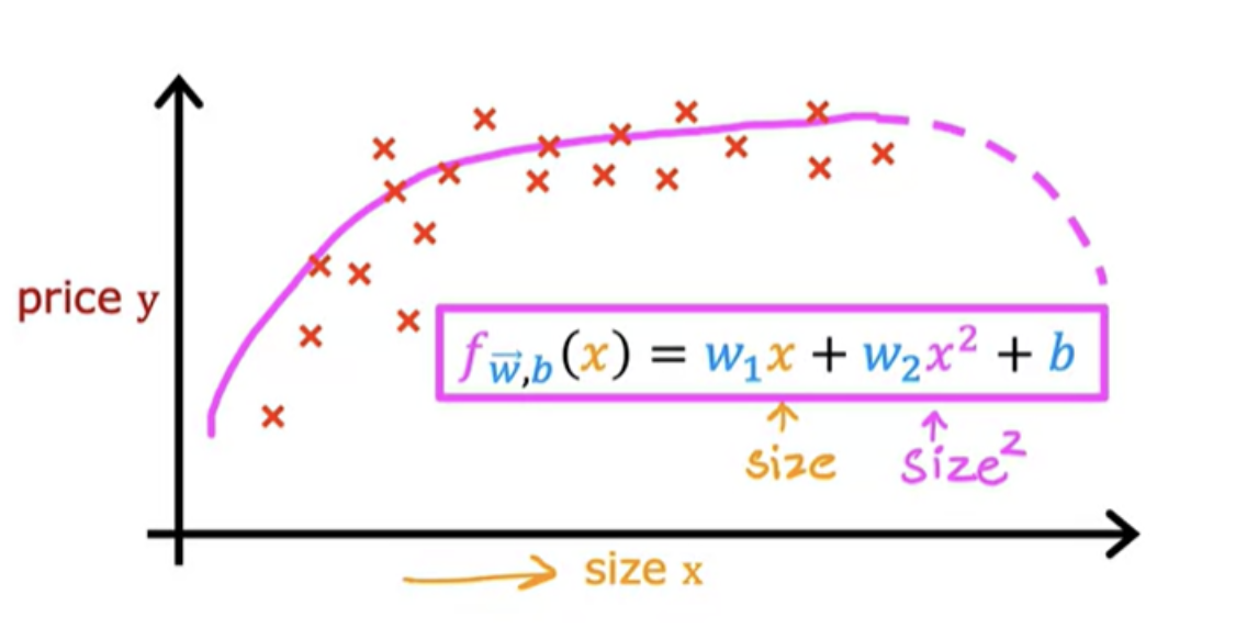
There is a flavor of feature engineering, that allow you to fit not just straight lines, but curves, non-linear functions to your data. Polynomial regression will let you fit curves, non-linear functions, to your data.
A polynomial is a general algebraic expression involving variables and coefficients, typically containing multiple terms and different powers of the variable. A quadratic is a specific type of polynomial where the highest power of the variable is 2, meaning it's a second-degree polynomial
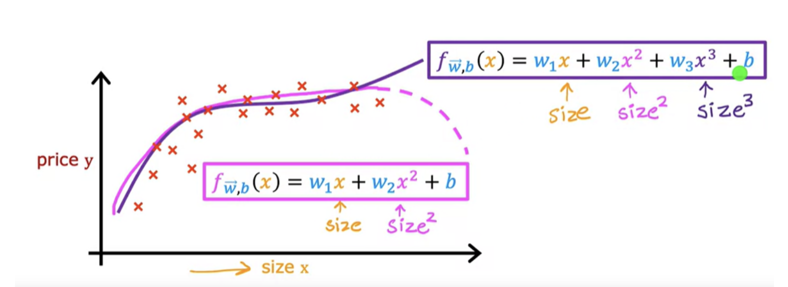
Sometimes quadratic model doesn't really make sense because a quadratic function eventually comes back down
A cubic function may be a better fit to the data because the size does eventually come back up as the size increases. In the case of the cubic function, the first feature is the size, the second feature is the size squared, and the third feature is the size cubed.
If you create features that are these powers like the square of the original features like this, then feature scaling becomes increasingly important. If the size of the house ranges from say, 1-1,000 square feet, then the second feature, which is a size squared, will range from one to a million, and the third feature, which is size cubed, ranges from one to a billion.
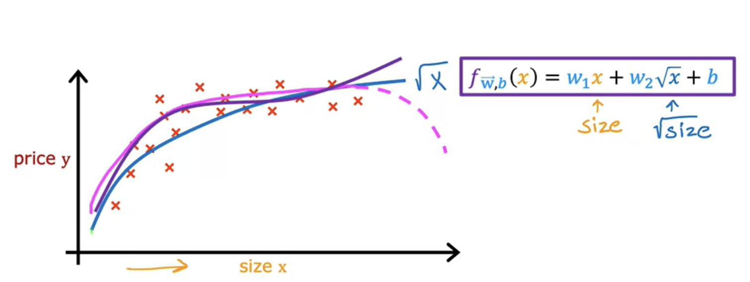
Another reasonable alternative to taking the size squared and size cubed is to say use the square root of x
In classification, output variable y can take on only one of a small handful of possible values instead of any number in an infinite range of numbers. Linear regression can be used to predict a number. Linear regression is not a good algorithm for classification problems. This will lead us into a different algorithm called logistic regression which is one of the most popular and most widely used learning algorithms today
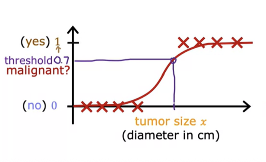
The type of classification problem where there are only two possible outputs is called binary classification. Example "Is this email a spam?", "Is the tumor is malignant?"
Linear regression predicts not just the values zero and one, but all numbers between zero and one or even less than zero or greater than one. But here we want to predict categories
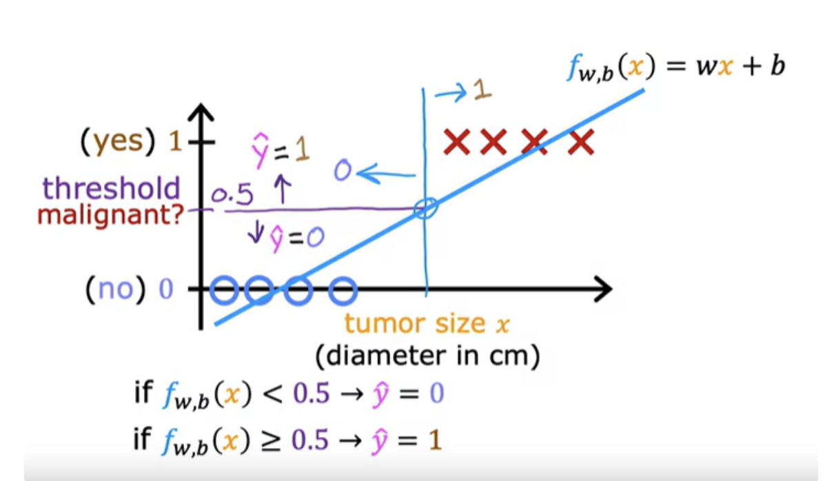
If you draw vertical line , everything to the left ends up with a prediction of y equals zero. And everything on the right ends up with the prediction of y equals one.
What happens if your dataset has one more training example (right side marked as x) ? Adding that example shouldn't change any of our conclusions about how to classify malignant versus benign tumors. When tumor is large, we want the algorithm to classify it as malignant
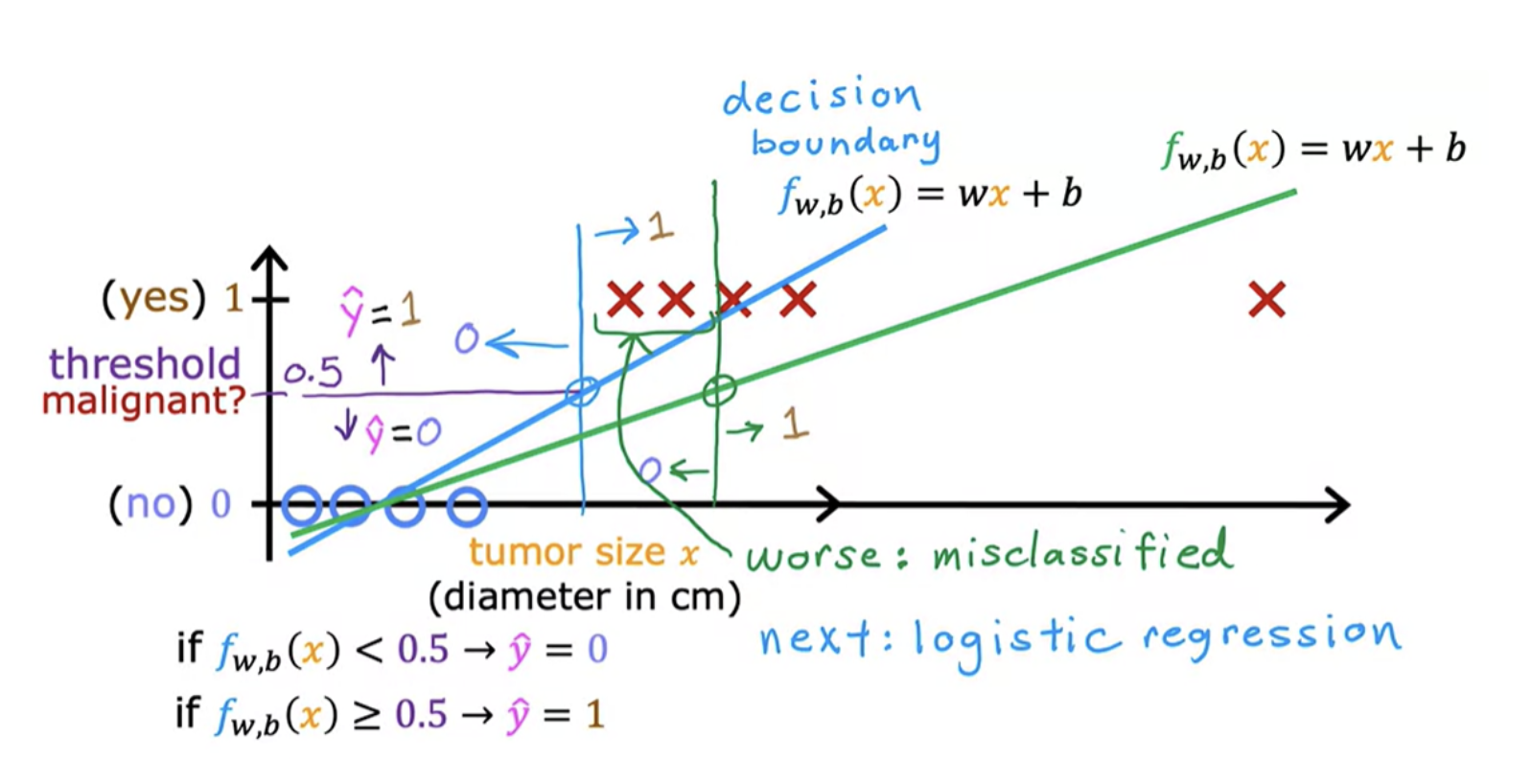
Logistic regression helps in this situation. Even though it has the word of regression in it is actually used for classification. The name was given for historical reasons. It is used to solve binary classification problems with output label y is either zero or one. In logistic regression we fit an S-shaped curve.
To build out to the logistic regression algorithm, there's an important mathematical function called the Sigmoid function, sometimes also referred to as the logistic function. It helps in outputing between 0 and 1.
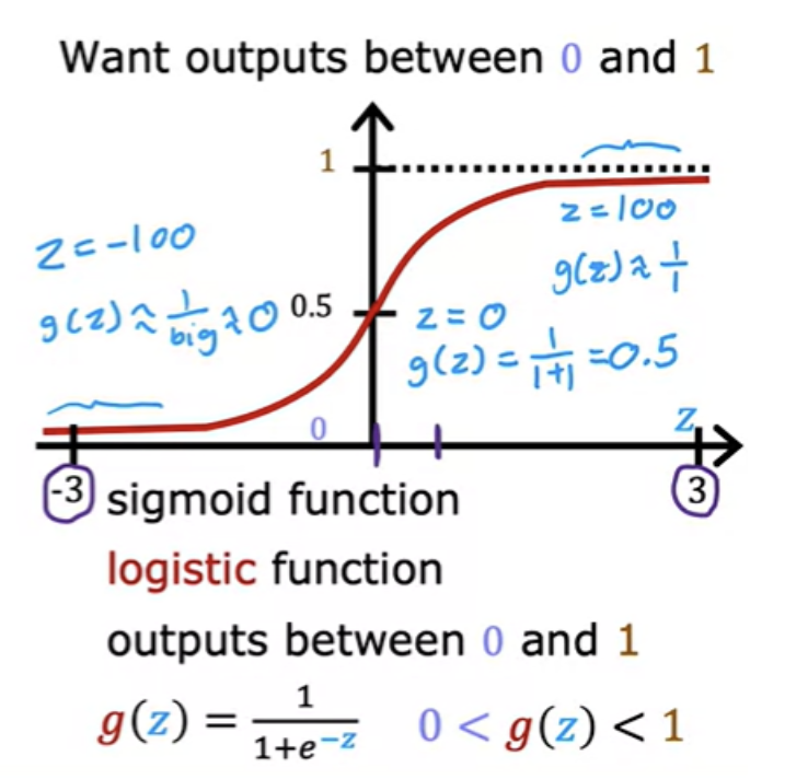
Horizontal axis takes on both negative and positive values here. "e" is a mathematical constant that takes on a value of about 2.7. When z is small (say -100) , g(z) will become closer to 0. When z is large (say 100), g(z) is going to be very close to 1.
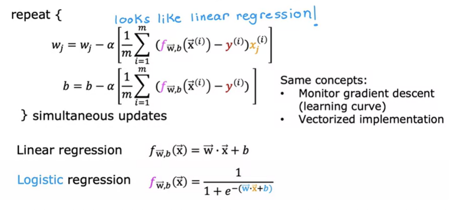
In linear regression, f(x) = w*x+b
In logistic regression, variable z refers to the linear combination of the input features and model parameters. It's the input to the sigmoid function Mathematicallyt it is
z = w*x+b
For example, x= hours predict if a student will pass based on study hours. x= hours studied, and predict whether the student passes (1) or fails (0). Let’s assume our model has learned: Weight: w=2, Bias: b=−4. Then
z= w*x+b = 2*3+(-4) = 2
Applying Sigmoid function g(z) = g(2) = 0.88. The model predicts a probability of 88% that the student will pass. If your threshold is 0.5, you'd classify this student as likely to pass.
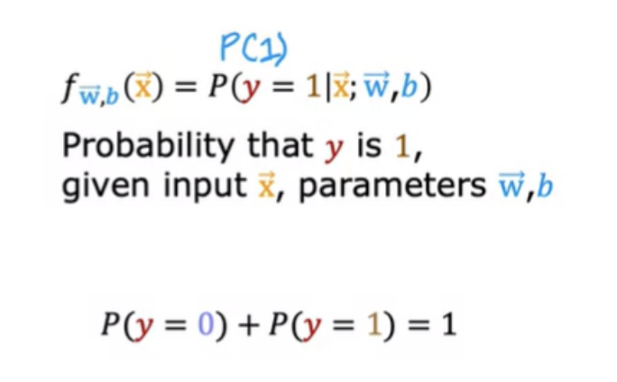
If the chance of y being 1 is 0.7 (70 percent), then the chance of it being 0 has got to be 0.3 (30 percent)
For a long time, a lot of Internet advertising was actually driven by a slight variation of logistic regression, that decided what ad was shown to you and many others on some large websites.
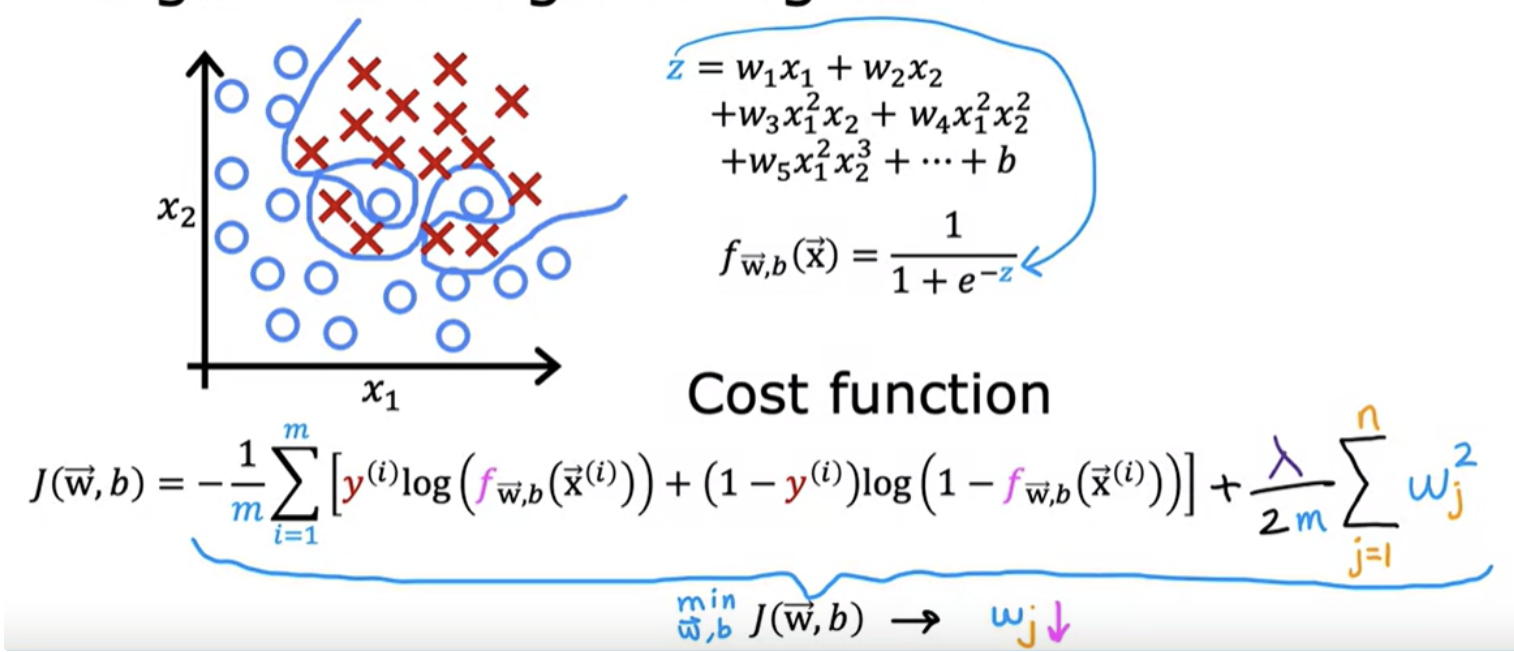
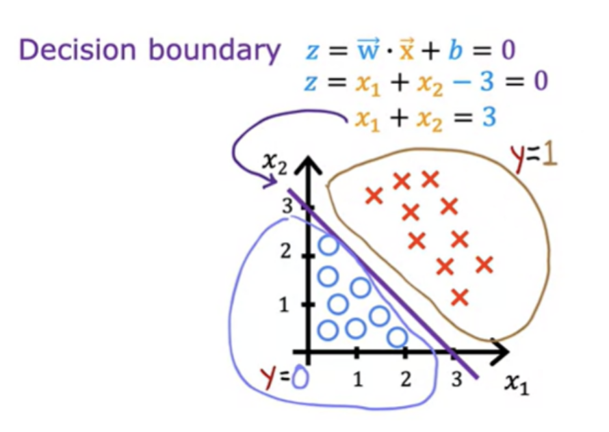
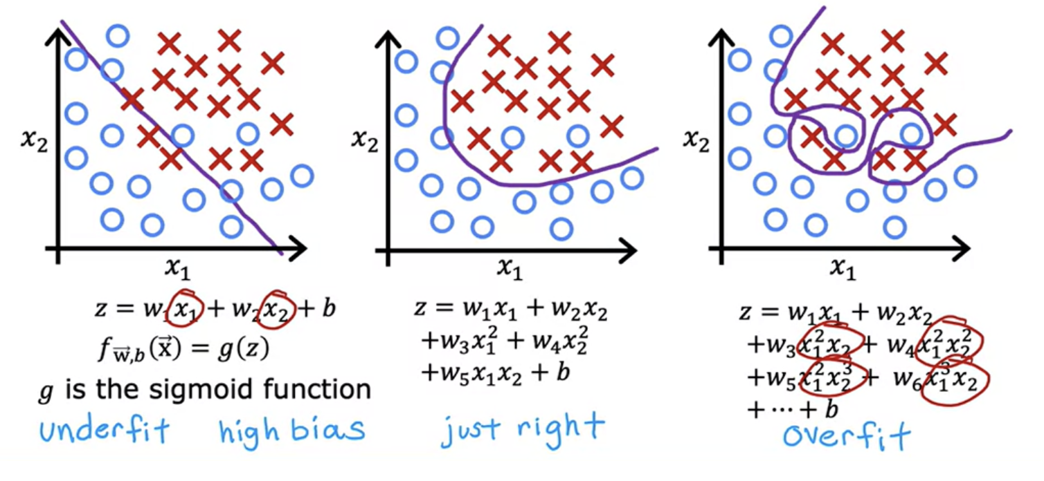
Here is a training set where the red crosses denote the positive examples and the blue circles denote negative examples The red crosses corresponds to y equals 1, and the blue circles correspond to y equals 0. Here decision boundary is a straight line.
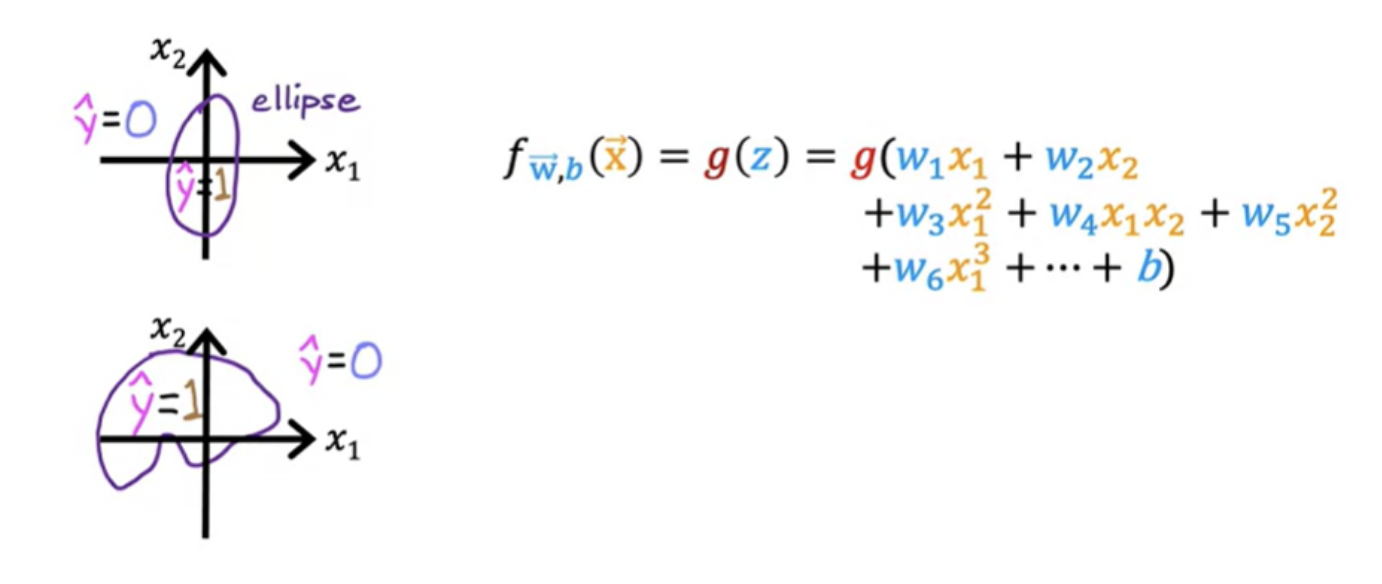
More complex examples may not have decision boundary as a straight line. It can be non-linear.
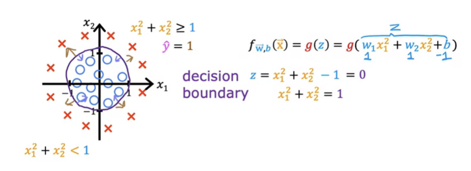
Even more complex decision boundaries can be made by even higher-order polynomial terms. Logistic regression can learn to fit pretty complex data.
Squared error cost function is not an ideal cost function for logistic regression. In linear regression, cost function looks like a convex function or a bowl shape or hammer shape. Now you could try to use the same cost function for logistic regression.
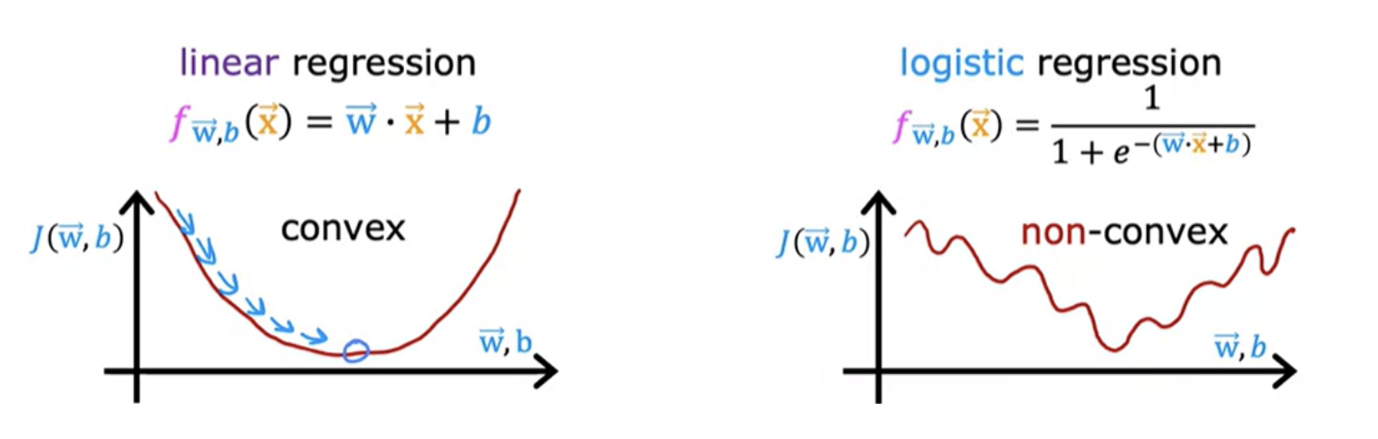
This becomes what's called a non-convex cost function. if you were to try to use gradient descent, there are lots of local minima that you can get into trouble. It turns out that for logistic regression, this squared error cost function is not a good choice. Instead, there will be a different cost function that can make the cost function convex again.
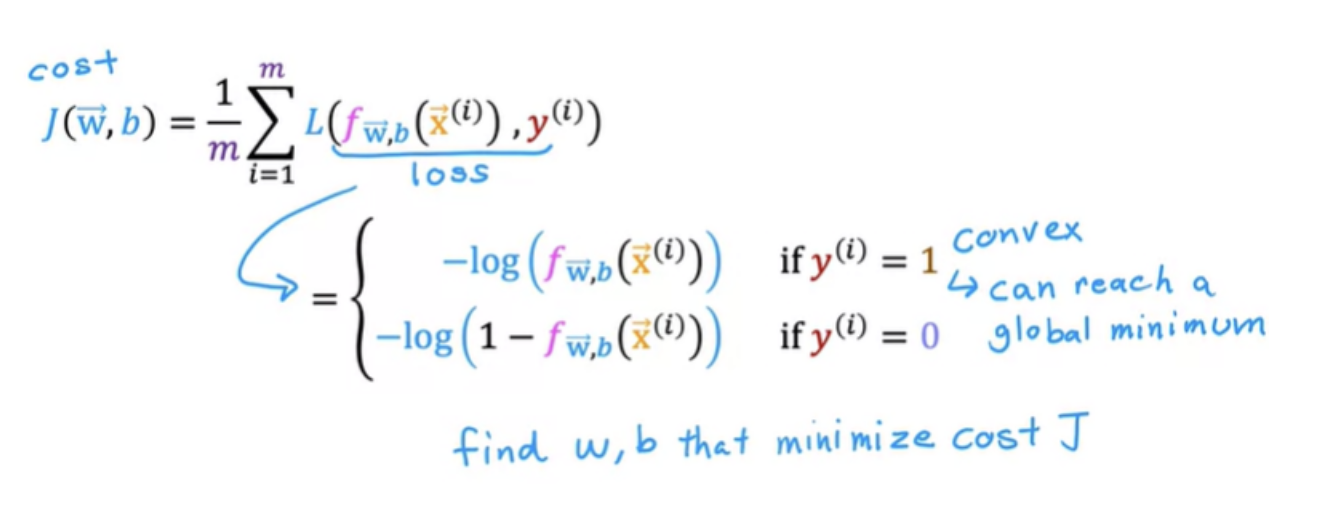
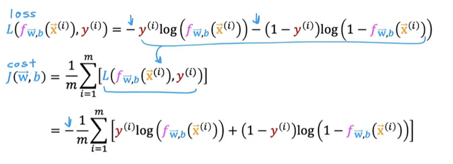
A loss function measures how well you're doing on one training example. By summing up the losses on all of the training examples you then get, the cost function, which measures how well you're doing on the entire training set.
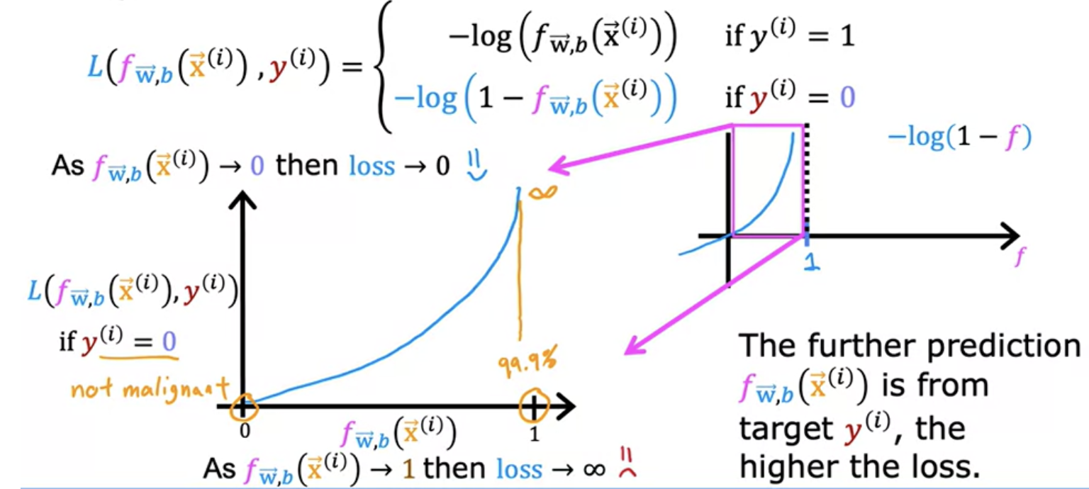
It turns out that with this choice of loss function, the overall cost function will be convex and thus you can reliably use gradient descent to take you to the global minimum
Cost function is a function of the entire training set and is, therefore, the average or 1 over m times the sum of the loss function on the individual training examples
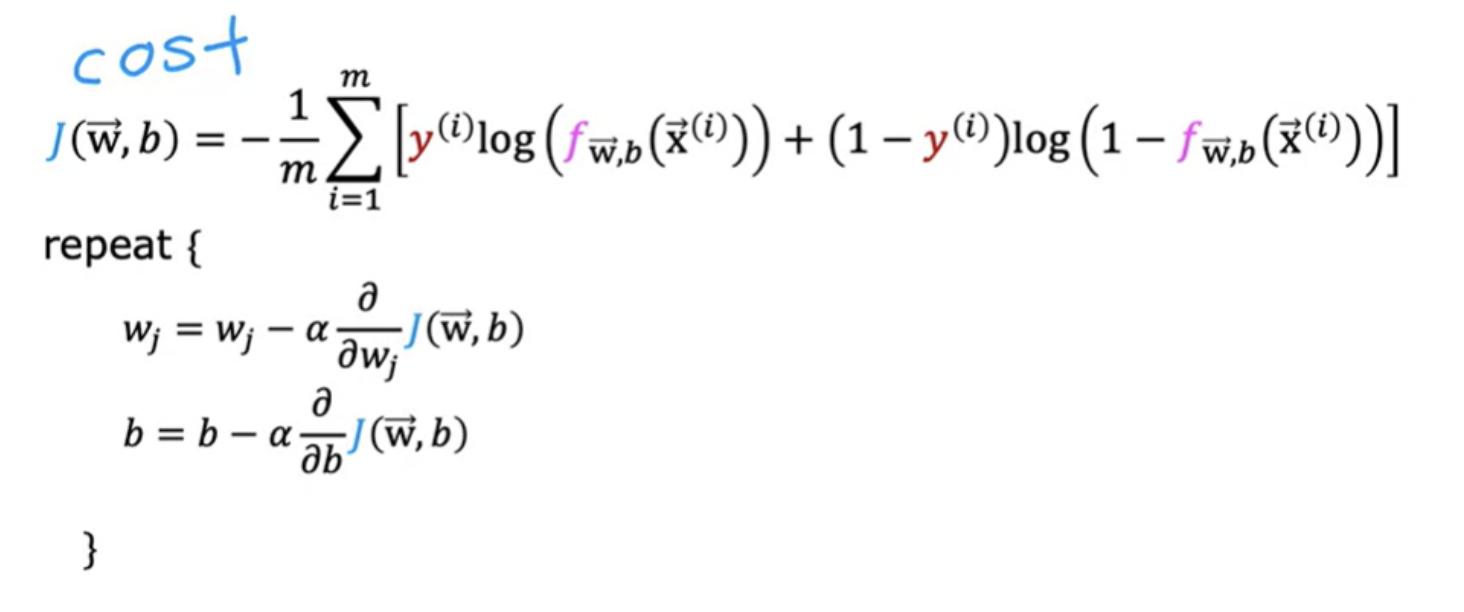
To fit the parameters of a logistic regression model , we have to find the values of the parameters w and b that minimize the cost function J.
In feature scaling for linear regression, we scaled all the features to take on similar ranges of values, say between negative 1 and plus 1. Feature scaling applied the same way to logistic regression to speed up gradient descent.
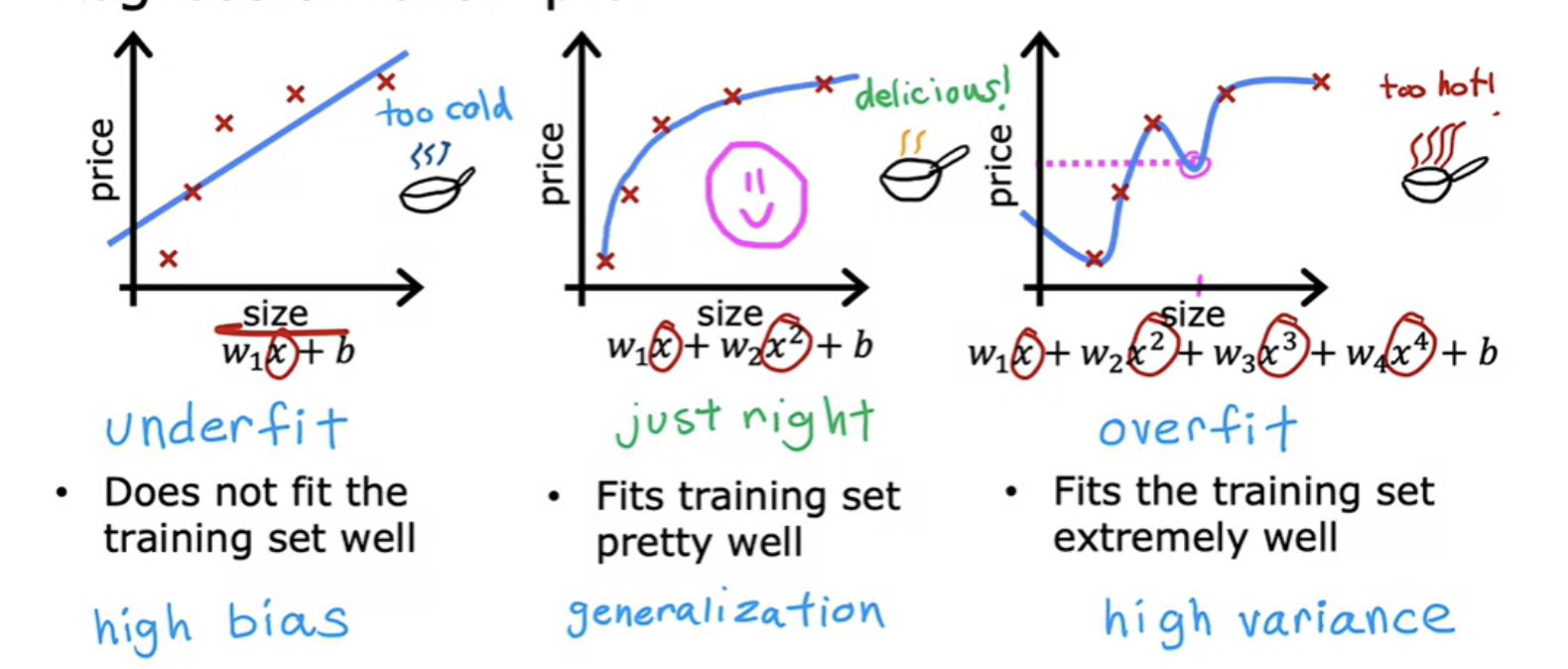
Underfitting means that the mode is just not even able to fit the training set that well. Another term for underfitting is the "algorithm has high bias".
A good fit is called generalize. Technically we say that you want your learning algorithm to generalize well, which means to make good predictions
Sometimes, the algorithm can run into a problem called overfitting, which can cause it to perform poorly. The model does extremely good job fitting the training data. It passes through all of the training data perfectly. The cost function being exactly equal to zero because the errors are zero.But this is a very wiggly curve, its going up and down all over the place. Another term for this is that the algorithm has high variance.In machine learning, many people will use the terms over-fit and high-variance almost interchangeably.
There are some techniques like regularization to help in minimizing overfitting problem and get the learning algorithms to work much better.
Overfitting applies a classification as well. For example classify if a tumor is malignant or benign.
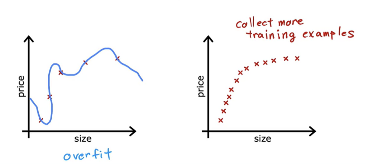
1. Collect more training examples
One way to address this problem is to collect more training data.With the larger training set, the learning algorithm will learn to fit a function that is less wiggly. You can continue to fit a high order polynomial or some of the function with a lot of features, and if you have enough training examples, it will still do okay.
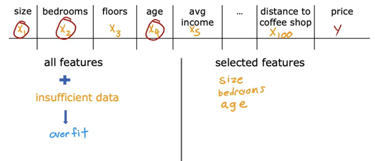
2. use fewer features
Getting more data isn't always an option. A second option for addressing overfitting is to see if you can use fewer features. If you have a lot of features but don't have enough training data, then your learning algorithm may also overfit to your training set.Choosing the most appropriate set of features to use is sometimes also called feature selection. One disadvantage of feature selection is that by using only a subset of the features, the algorithm is throwing away some of the information. Regularization is a way to more gently reduce the impacts of some of the features without doing something as harsh as eliminating it outright
3. Regularisation
Regularisation lets you keep all of your features, but they just prevents the features from having an overly large effect, which is what sometimes can cause overfitting. It reduces the size of the parameters. Regularization is a very frequently used technique.
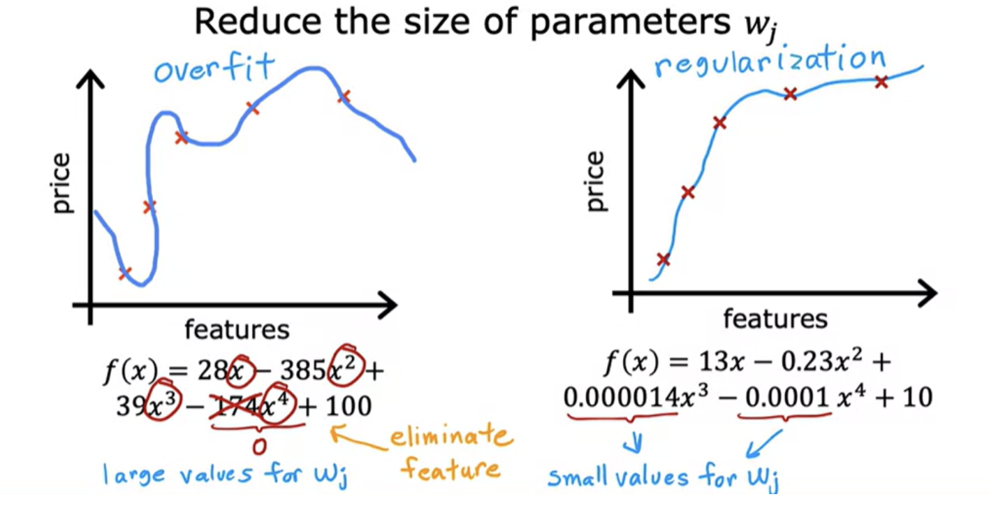
If you fit a quadratic function to a sample data, it gives a pretty good fit. But if you fit a very high order polynomial, you end up with a curve that over fits the data
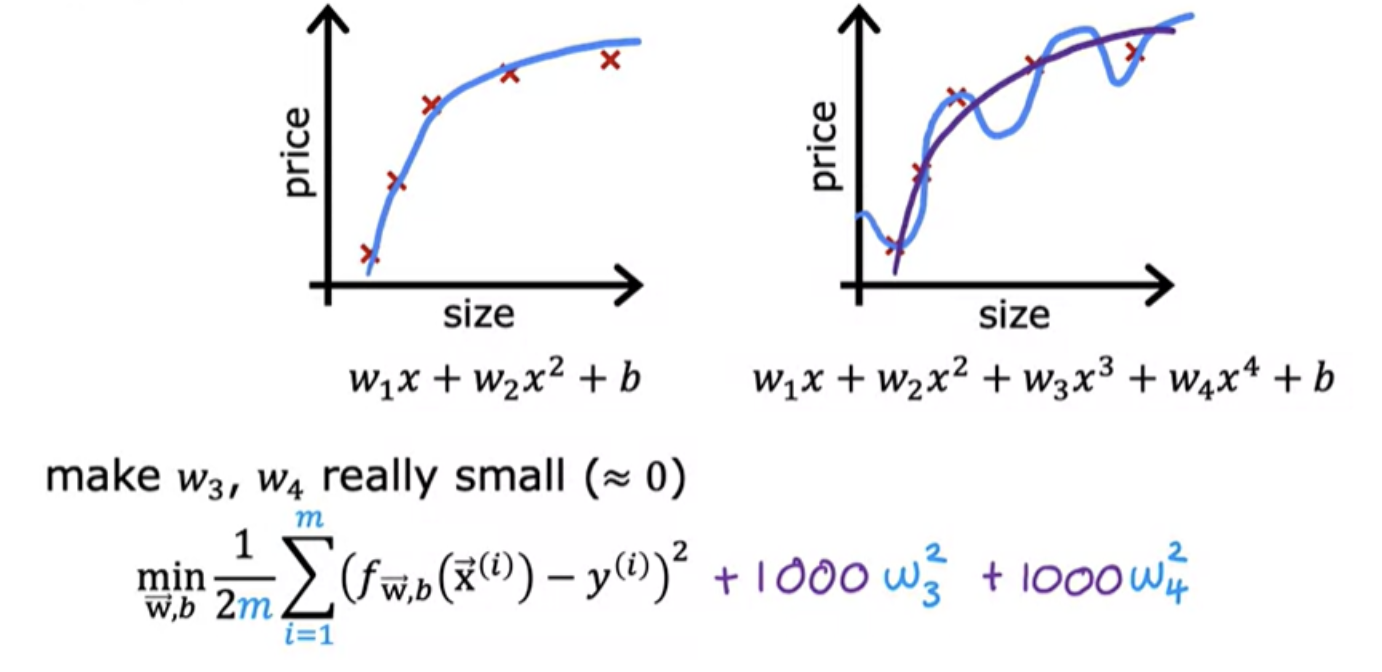
In the above example 1000 is chosen as a larger number.So with this modified cost function, you are penalizing the model if w3 and w4 are large. Because if you want to minimize this function, the only way to make this new cost function small is if w3 and w4 are both small. So when you minimize this function, you are going to end up with w3 close to 0 and w4 close to 0. So we're effectively nearly canceling out the effects of the features x 3 and x 4 and getting rid of these two terms. The idea is that if there are smaller values for the parameters, then that's a bit like having a simpler model.
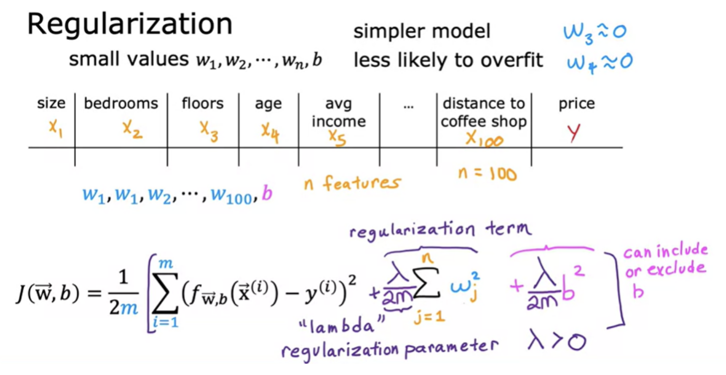
If you have a lot of features, say a 100 features, you may not know which are the most important features and which ones to penalize. So the way regularization is typically implemented is to penalize all of the features. Let's penalize all of them a bit and shrink all of them by adding this new term lambda.We also divide lambda by 2m so that both the 1st and 2nd terms here are scaled by 1/2m.
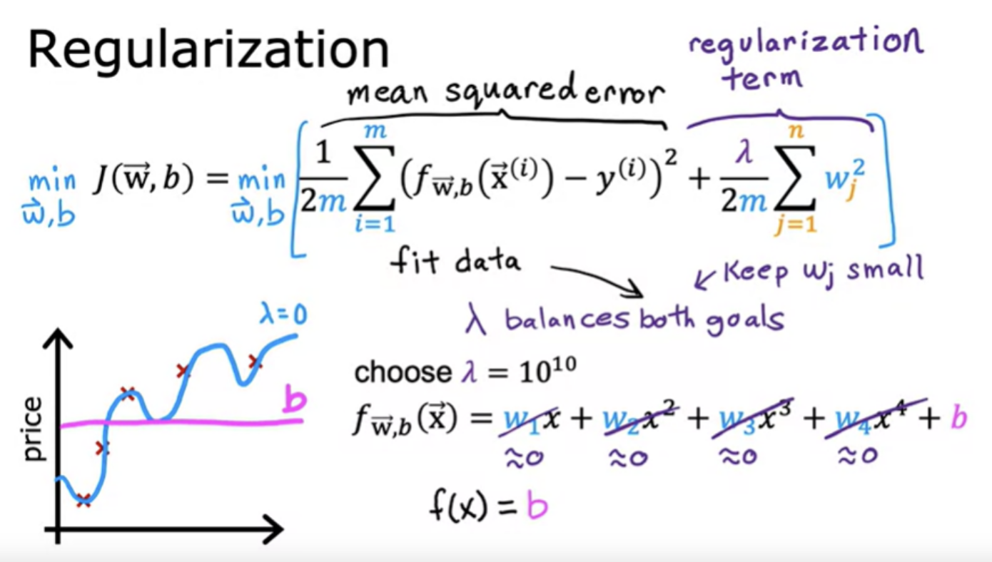
If lambda is very, very large, the learning algorithm will choose w1, w2, w3 and w4 to be extremely close to 0 and thus f(x) is basically equal to b and so the learning algorithm fits a horizontal straight line and under fits
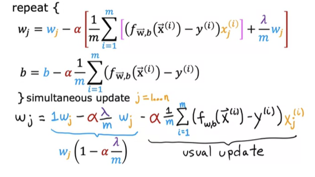
What regularization is doing on every single iteration is you're multiplying w by a number slightly less than 1 and that has effect of shrinking the value of wj just a little bit
Gradient update for logistic regression is similar to the gradient update for linear regression. Similarly the gradient descent update for regularized logistic regression will also look similar to the update for regularized linear regression